
使用transformer进行图像分类
文章目录
1、导入模型
2、定义加载函数
3、定义批量加载函数
4、加载数据
5、定义数据预处理及训练模型的一些超参数
6、定义数据增强模型
7、构建模型
7.1 构建多层感知器(MLP)
7.2 创建一个类似卷积层的patch层
7.3 查看由patch层随机生成的图像块
7.4构建patch 编码层( encoding layer)
7.5构建ViT模型
8、编译、训练模型
9、查看运行结果
使用Transformer来提升模型的性能
最近几年,Transformer体系结构已成为自然语言处理任务的实际标准,
但其在计算机视觉中的应用还受到限制。在视觉上,注意力要么与卷积网络结合使用,
要么用于替换卷积网络的某些组件,同时将其整体结构保持在适当的位置。2020年10月22日,谷歌人工智能研究院发表一篇题为“An Image is Worth 16x16 Words: Transformers for Image Recognition at Scale”的文章。文章将图像切割成一个个图像块,组成序列化的数据输入Transformer执行图像分类任务。当对大量数据进行预训练并将其传输到多个中型或小型图像识别数据集(如ImageNet、CIFAR-100、VTAB等)时,与目前的卷积网络相比,Vision Transformer(ViT)获得了出色的结果,同时所需的计算资源也大大减少。
这里我们以ViT我模型,实现对数据CiFar10的分类工作,模型性能得到进一步的提升。
1、导入模型
import osimport mathimport numpy as npimport pickle as pimport tensorflow as tffrom tensorflow import kerasimport matplotlib.pyplot as pltfrom tensorflow.keras import layersimport tensorflow_addons as tfa%matplotlib inline
这里使用了TensorFlow_addons模块,它实现了核心 TensorFlow 中未提供的新功能。
tensorflow_addons的安装要注意与tf的版本对应关系,请参考:
https://github.com/tensorflow/addons。
安装addons时要注意其版本与tensorflow版本的对应,具体关系以上这个链接有。
2、定义加载函数
def load_CIFAR_data(data_dir):"""load CIFAR data"""images_train=[]labels_train=[]for i in range(5):f=os.path.join(data_dir,'data_batch_%d' % (i+1))print('loading ',f)# 调用 load_CIFAR_batch( )获得批量的图像及其对应的标签image_batch,label_batch=load_CIFAR_batch(f)images_train.append(image_batch)labels_train.append(label_batch)Xtrain=np.concatenate(images_train)Ytrain=np.concatenate(labels_train)del image_batch ,label_batchXtest,Ytest=load_CIFAR_batch(os.path.join(data_dir,'test_batch'))print('finished loadding CIFAR-10 data')# 返回训练集的图像和标签,测试集的图像和标签return (Xtrain,Ytrain),(Xtest,Ytest)
3、定义批量加载函数
def load_CIFAR_batch(filename):""" load single batch of cifar """with open(filename, 'rb')as f:# 一个样本由标签和图像数据组成# (3072=32x32x3)# ...#data_dict = p.load(f, encoding='bytes')images= data_dict[b'data']labels = data_dict[b'labels']# 把原始数据结构调整为: BCWHimages = images.reshape(10000, 3, 32, 32)# tensorflow处理图像数据的结构:BWHC# 把通道数据C移动到最后一个维度images = images.transpose (0,2,3,1)labels = np.array(labels)return images, labels
4、加载数据
data_dir = r'C:\Users\wumg\jupyter-ipynb\data\cifar-10-batches-py'(x_train,y_train),(x_test,y_test) = load_CIFAR_data(data_dir)
把数据转换为dataset格式
train_dataset = tf.data.Dataset.from_tensor_slices((x_train, y_train))test_dataset = tf.data.Dataset.from_tensor_slices((x_test, y_test))
5、定义数据预处理及训练模型的一些超参数
num_classes = 10input_shape = (32, 32, 3)learning_rate = 0.001weight_decay = 0.0001batch_size = 256num_epochs = 10image_size = 72 # We'll resize input images to this sizepatch_size = 6 # Size of the patches to be extract from the input imagesnum_patches = (image_size // patch_size) ** 2projection_dim = 64num_heads = 4transformer_units = [projection_dim * 2,projection_dim,] # Size of the transformer layerstransformer_layers = 8mlp_head_units = [2048, 1024] # Size of the dense layers of the final classifier
6、定义数据增强模型
data_augmentation = keras.Sequential([layers.experimental.preprocessing.Normalization(),layers.experimental.preprocessing.Resizing(image_size, image_size),layers.experimental.preprocessing.RandomFlip("horizontal"),layers.experimental.preprocessing.RandomRotation(factor=0.02),layers.experimental.preprocessing.RandomZoom(height_factor=0.2, width_factor=0.2),],name="data_augmentation",)# 使预处理层的状态与正在传递的数据相匹配#Compute the mean and the variance of the training data for normalization.data_augmentation.layers[0].adapt(x_train)
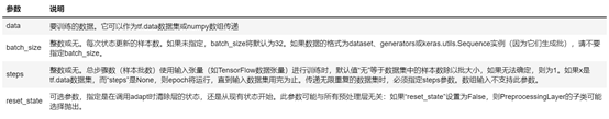
预处理层是在模型训练开始之前计算其状态的层。他们在训练期间不会得到更新。大多数预处理层为状态计算实现了adapt()方法。
adapt(data, batch_size=None, steps=None, reset_state=True)该函数参数说明如下:
7、构建模型
7.1 构建多层感知器(MLP)
def mlp(x, hidden_units, dropout_rate):for units in hidden_units:x = layers.Dense(units, activation=tf.nn.gelu)(x)x = layers.Dropout(dropout_rate)(x)return x
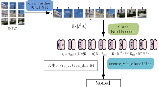
7.2 创建一个类似卷积层的patch层
class Patches(layers.Layer):def __init__(self, patch_size):super(Patches, self).__init__()self.patch_size = patch_sizedef call(self, images):batch_size = tf.shape(images)[0]patches = tf.image.extract_patches(images=images,sizes=[1, self.patch_size, self.patch_size, 1],strides=[1, self.patch_size, self.patch_size, 1],rates=[1, 1, 1, 1],padding="VALID",)patch_dims = patches.shape[-1]patches = tf.reshape(patches, [batch_size, -1, patch_dims])return patches
7.3 查看由patch层随机生成的图像块
import matplotlib.pyplot as pltplt.figure(figsize=(4, 4))image = x_train[np.random.choice(range(x_train.shape[0]))]plt.imshow(image.astype("uint8"))plt.axis("off")resized_image = tf.image.resize(tf.convert_to_tensor([image]), size=(image_size, image_size))patches = Patches(patch_size)(resized_image)print(f"Image size: {image_size} X {image_size}")print(f"Patch size: {patch_size} X {patch_size}")print(f"Patches per image: {patches.shape[1]}")print(f"Elements per patch: {patches.shape[-1]}")n = int(np.sqrt(patches.shape[1]))plt.figure(figsize=(4, 4))for i, patch in enumerate(patches[0]):ax = plt.subplot(n, n, i + 1)patch_img = tf.reshape(patch, (patch_size, patch_size, 3))plt.imshow(patch_img.numpy().astype("uint8"))plt.axis("off")
运行结果
Image size: 72 X 72
Patch size: 6 X 6
Patches per image: 144
Elements per patch: 108


7.4构建patch 编码层( encoding layer)
class PatchEncoder(layers.Layer):def __init__(self, num_patches, projection_dim):super(PatchEncoder, self).__init__()self.num_patches = num_patches#一个全连接层,其输出维度为projection_dim,没有指明激活函数self.projection = layers.Dense(units=projection_dim)#定义一个嵌入层,这是一个可学习的层#输入维度为num_patches,输出维度为projection_dimself.position_embedding = layers.Embedding(input_dim=num_patches, output_dim=projection_dim)def call(self, patch):positions = tf.range(start=0, limit=self.num_patches, delta=1)encoded = self.projection(patch) + self.position_embedding(positions)return encoded
7.5构建ViT模型
def create_vit_classifier():inputs = layers.Input(shape=input_shape)# Augment data.augmented = data_augmentation(inputs)#augmented = augmented_train_batches(inputs)# Create patches.patches = Patches(patch_size)(augmented)# Encode patches.encoded_patches = PatchEncoder(num_patches, projection_dim)(patches)# Create multiple layers of the Transformer block.for _ in range(transformer_layers):# Layer normalization 1.x1 = layers.LayerNormalization(epsilon=1e-6)(encoded_patches)# Create a multi-head attention layer.attention_output = layers.MultiHeadAttention(num_heads=num_heads, key_dim=projection_dim, dropout=0.1x1)# Skip connection 1.x2 = layers.Add()([attention_output, encoded_patches])# Layer normalization 2.x3 = layers.LayerNormalization(epsilon=1e-6)(x2)# MLP.x3 = mlp(x3, hidden_units=transformer_units, dropout_rate=0.1)# Skip connection 2.encoded_patches = layers.Add()([x3, x2])# Create a [batch_size, projection_dim] tensor.representation = layers.LayerNormalization(epsilon=1e-6)(encoded_patches)representation = layers.Flatten()(representation)representation = layers.Dropout(0.5)(representation)# Add MLP.features = mlp(representation, hidden_units=mlp_head_units, dropout_rate=0.5)# Classify outputs.logits = layers.Dense(num_classes)(features)# Create the Keras model.model = keras.Model(inputs=inputs, outputs=logits)return model
该模型的处理流程如下图所示
8、编译、训练模型
def run_experiment(model):optimizer = tfa.optimizers.AdamW(learning_rate=learning_rate, weight_decay=weight_decay)model.compile(optimizer=optimizer,loss=keras.losses.SparseCategoricalCrossentropy(from_logits=True),metrics=[="accuracy"),name="top-5-accuracy"),],)#checkpoint_filepath = r".\tmp\checkpoint"checkpoint_filepath ="model_bak.hdf5"checkpoint_callback = keras.callbacks.ModelCheckpoint(checkpoint_filepath,monitor="val_accuracy",save_best_only=True,save_weights_only=True,)history = model.fit(x=x_train,y=y_train,batch_size=batch_size,epochs=num_epochs,validation_split=0.1,callbacks=[checkpoint_callback],)model.load_weights(checkpoint_filepath)accuracy, top_5_accuracy = model.evaluate(x_test, y_test)accuracy: {round(accuracy * 100, 2)}%")top 5 accuracy: {round(top_5_accuracy * 100, 2)}%")return history
实例化类,运行模型
vit_classifier = create_vit_classifier()history = run_experiment(vit_classifier)
运行结果
Epoch 1/10
176/176 [==============================] - 68s 333ms/step - loss: 2.6394 - accuracy: 0.2501 - top-5-accuracy: 0.7377 - val_loss: 1.5331 - val_accuracy: 0.4580 - val_top-5-accuracy: 0.9092
Epoch 2/10
176/176 [==============================] - 58s 327ms/step - loss: 1.6359 - accuracy: 0.4150 - top-5-accuracy: 0.8821 - val_loss: 1.2714 - val_accuracy: 0.5348 - val_top-5-accuracy: 0.9464
Epoch 3/10
176/176 [==============================] - 58s 328ms/step - loss: 1.4332 - accuracy: 0.4839 - top-5-accuracy: 0.9210 - val_loss: 1.1633 - val_accuracy: 0.5806 - val_top-5-accuracy: 0.9616
Epoch 4/10
176/176 [==============================] - 58s 329ms/step - loss: 1.3253 - accuracy: 0.5280 - top-5-accuracy: 0.9349 - val_loss: 1.1010 - val_accuracy: 0.6112 - val_top-5-accuracy: 0.9572
Epoch 5/10
176/176 [==============================] - 58s 330ms/step - loss: 1.2380 - accuracy: 0.5626 - top-5-accuracy: 0.9411 - val_loss: 1.0212 - val_accuracy: 0.6400 - val_top-5-accuracy: 0.9690
Epoch 6/10
176/176 [==============================] - 58s 330ms/step - loss: 1.1486 - accuracy: 0.5945 - top-5-accuracy: 0.9520 - val_loss: 0.9698 - val_accuracy: 0.6602 - val_top-5-accuracy: 0.9718
Epoch 7/10
176/176 [==============================] - 58s 330ms/step - loss: 1.1208 - accuracy: 0.6060 - top-5-accuracy: 0.9558 - val_loss: 0.9215 - val_accuracy: 0.6724 - val_top-5-accuracy: 0.9790
Epoch 8/10
176/176 [==============================] - 58s 330ms/step - loss: 1.0643 - accuracy: 0.6248 - top-5-accuracy: 0.9621 - val_loss: 0.8709 - val_accuracy: 0.6944 - val_top-5-accuracy: 0.9768
Epoch 9/10
176/176 [==============================] - 58s 330ms/step - loss: 1.0119 - accuracy: 0.6446 - top-5-accuracy: 0.9640 - val_loss: 0.8290 - val_accuracy: 0.7142 - val_top-5-accuracy: 0.9784
Epoch 10/10
176/176 [==============================] - 58s 330ms/step - loss: 0.9740 - accuracy: 0.6615 - top-5-accuracy: 0.9666 - val_loss: 0.8175 - val_accuracy: 0.7096 - val_top-5-accuracy: 0.9806
313/313 [==============================] - 9s 27ms/step - loss: 0.8514 - accuracy: 0.7032 - top-5-accuracy: 0.9773
Test accuracy: 70.32%
Test top 5 accuracy: 97.73%
In [15]:
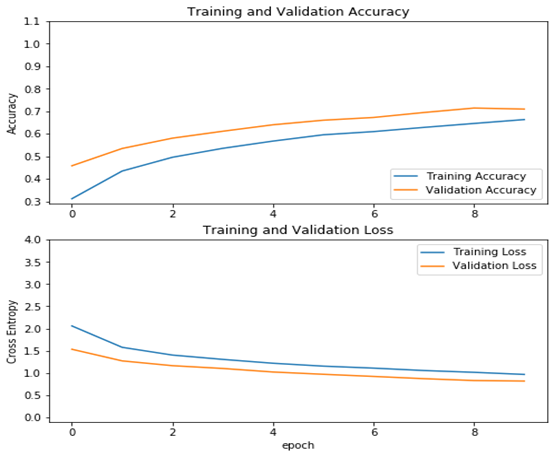
从结果看可以来看,测试精度已达70%,这是一个较大提升!
9、查看运行结果
acc = history.history['accuracy']val_acc = history.history['val_accuracy']loss = history.history['loss']val_loss =history.history['val_loss']plt.figure(figsize=(8, 8))plt.subplot(2, 1, 1)plt.plot(acc, label='Training Accuracy')plt.plot(val_acc, label='Validation Accuracy')plt.legend(loc='lower right')plt.ylabel('Accuracy')plt.ylim([min(plt.ylim()),1.1])plt.title('Training and Validation Accuracy')plt.subplot(2, 1, 2)plt.plot(loss, label='Training Loss')plt.plot(val_loss, label='Validation Loss')plt.legend(loc='upper right')plt.ylabel('Cross Entropy')plt.ylim([-0.1,4.0])plt.title('Training and Validation Loss')plt.xlabel('epoch')plt.show()
运行结果
作者 :吴茂贵,资深大数据和人工智能技术专家,在BI、数据挖掘与分析、数据仓库、机器学习等领域工作超过20年!在基于Spark、TensorFlow、Pytorch、Keras等机器学习和深度学习方面有大量的工程实践经验。代表作有《深入浅出Embedding:原理解析与应用实践》、《Python深度学习基于Pytorch》和《Python深度学习基于TensorFlow》。
——The End——


点击购买