来源：DeepHub IMBA

本文约3600字，建议阅读9分钟

本文手把手教你小样本学习方法。

什么是小样本学习？

1. N-Shot Learning (NSL)
2. Few-Shot Learning ( FSL )
3. One-Shot Learning (OSL)
4. Zero-Shot Learning (ZSL)

小样本学习方法

小样本学习图像分类算法

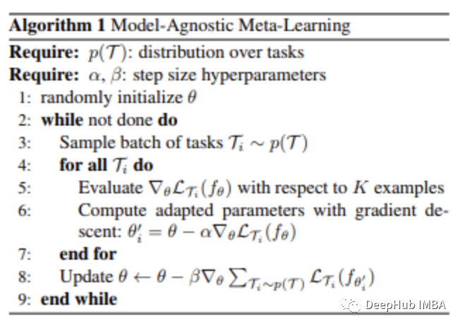
1. 元学习者在每个分集（episode）开始时创建自己的副本C，
2. C 在这一分集上进行训练（在 base-model 的帮助下），
3. C 对查询集进行预测，
4. 从这些预测中计算出的损失用于更新 C，
5. 这种情况一直持续到完成所有分集的训练。

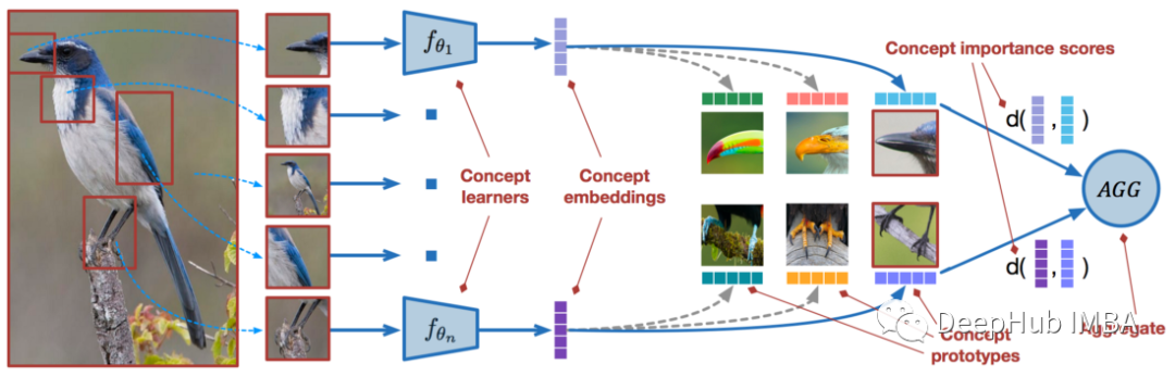
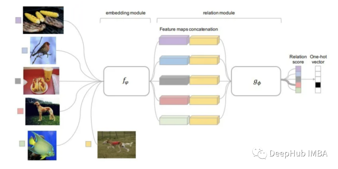
• 来自支持集和查询集的每个图像都被馈送到一个 CNN，该 CNN 为它们输出特征的嵌入
• 查询图像使用支持集训练的模型得到嵌入特征的余弦距离，通过 softmax 进行分类
• 分类结果的交叉熵损失通过 CNN 反向传播更新特征嵌入模型

使用 Open-AI Clip 进行零样本学习

 ! pip install ftfy regex tqdm ! pip install git+https://github.com/openai/CLIP.gitimport numpy as np import torch from pkg_resources import packaging
 print("Torch version:", torch.__version__)

 import clipclip.available_models() # it will list the names of available CLIP modelsmodel, preprocess = clip.load("ViT-B/32") model.cuda().eval() input_resolution = model.visual.input_resolution context_length = model.context_length vocab_size = model.vocab_size
 print("Model parameters:", f"{np.sum([int(np.prod(p.shape)) for p in model.parameters()]):,}") print("Input resolution:", input_resolution) print("Context length:", context_length) print("Vocab size:", vocab_size)

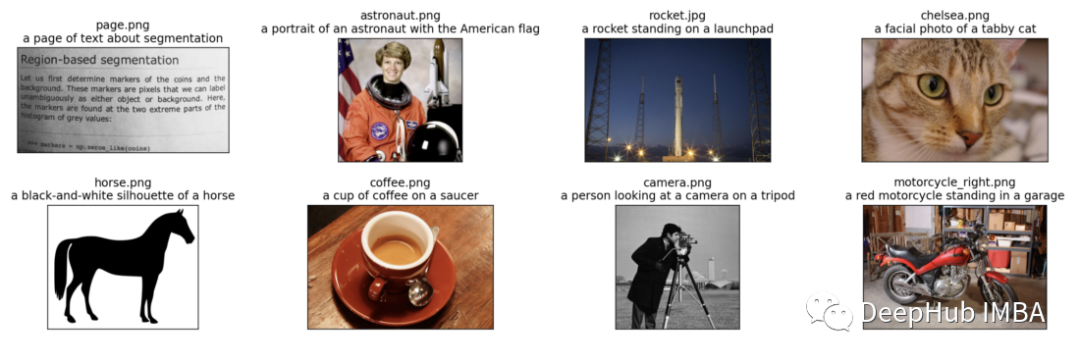
 import os import skimage import IPython.display import matplotlib.pyplot as plt from PIL import Image import numpy as np
 from collections import OrderedDict import torch
 %matplotlib inline %config InlineBackend.figure_format = 'retina'
 # images in skimage to use and their textual descriptions descriptions = {    "page": "a page of text about segmentation",    "chelsea": "a facial photo of a tabby cat",    "astronaut": "a portrait of an astronaut with the American flag",    "rocket": "a rocket standing on a launchpad",    "motorcycle_right": "a red motorcycle standing in a garage",    "camera": "a person looking at a camera on a tripod",    "horse": "a black-and-white silhouette of a horse",    "coffee": "a cup of coffee on a saucer" }original_images = [] images = [] texts = [] plt.figure(figsize=(16, 5))
 for filename in [filename for filename in os.listdir(skimage.data_dir) if filename.endswith(".png") or filename.endswith(".jpg")]:    name = os.path.splitext(filename)[0]    if name not in descriptions:        continue
    image = Image.open(os.path.join(skimage.data_dir, filename)).convert("RGB")
    plt.subplot(2, 4, len(images) + 1)    plt.imshow(image)    plt.title(f"{filename}\n{descriptions[name]}")    plt.xticks([])    plt.yticks([])
    original_images.append(image)    images.append(preprocess(image))    texts.append(descriptions[name])
 plt.tight_layout()

 image_input = torch.tensor(np.stack(images)).cuda() text_tokens = clip.tokenize(["This is " + desc for desc in texts]).cuda()
 with torch.no_grad():    image_features = model.encode_image(image_input).float()    text_features = model.encode_text(text_tokens).float()

 image_features /= image_features.norm(dim=-1, keepdim=True) text_features /= text_features.norm(dim=-1, keepdim=True) similarity = text_features.cpu().numpy() @ image_features.cpu().numpy().T
 count = len(descriptions)
 plt.figure(figsize=(20, 14)) plt.imshow(similarity, vmin=0.1, vmax=0.3) # plt.colorbar() plt.yticks(range(count), texts, fontsize=18) plt.xticks([]) for i, image in enumerate(original_images):    plt.imshow(image, extent=(i - 0.5, i + 0.5, -1.6, -0.6), origin="lower") for x in range(similarity.shape[1]):    for y in range(similarity.shape[0]):        plt.text(x, y, f"{similarity[y, x]:.2f}", ha="center", va="center", size=12)
 for side in ["left", "top", "right", "bottom"]:  plt.gca().spines[side].set_visible(False)
 plt.xlim([-0.5, count - 0.5]) plt.ylim([count + 0.5, -2])
 plt.title("Cosine similarity between text and image features", size=20)

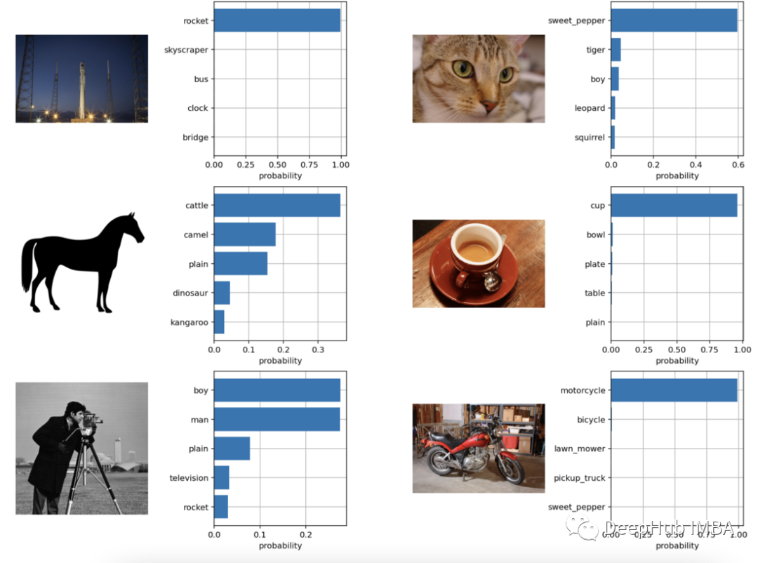
 from torchvision.datasets import CIFAR100 cifar100 = CIFAR100(os.path.expanduser("~/.cache"), transform=preprocess, download=True) text_descriptions = [f"This is a photo of a {label}" for label in cifar100.classes] text_tokens = clip.tokenize(text_descriptions).cuda() with torch.no_grad():    text_features = model.encode_text(text_tokens).float()    text_features /= text_features.norm(dim=-1, keepdim=True)
 text_probs = (100.0 * image_features @ text_features.T).softmax(dim=-1) top_probs, top_labels = text_probs.cpu().topk(5, dim=-1) plt.figure(figsize=(16, 16)) for i, image in enumerate(original_images):    plt.subplot(4, 4, 2 * i + 1)    plt.imshow(image)    plt.axis("off")
    plt.subplot(4, 4, 2 * i + 2)    y = np.arange(top_probs.shape[-1])    plt.grid()    plt.barh(y, top_probs[i])    plt.gca().invert_yaxis()    plt.gca().set_axisbelow(True)    plt.yticks(y, [cifar100.classes[index] for index in top_labels[i].numpy()])    plt.xlabel("probability")
 plt.subplots_adjust(wspace=0.5) plt.show()