
【深度学习】实战教程 | 车道线检测项目实战,霍夫变换 & 新方法 Spatial CNN
此文按照这样的逻辑进行撰写。分享机器学习、计算机视觉的基础知识,接着我们以一个实际的项目,带领大家自己动手实践。最后,分享更多学习资料、进阶项目实战,这部分属于我CSDN上的专栏,最后会按照顺序给出相应的链接,供大家选择学习。
理论篇:算法基础(可选择后看)
本专栏所涉及的项目所需机器学习/图像处理知识并不深入,但我之前在CSDN也开设了《机器学习算法讲解与Python实现》和《计算机视觉前沿论文研读》两个专栏。一个更偏算法理论,一个则关注于计算机视觉顶会的前沿论文成果,解读新的方法和Idea。
《机器学习算法讲解与Python实现》
专栏链接 https://blog.csdn.net/charmve/category_9657673.html
《计算机视觉前沿论文研读》

专栏链接 https://blog.csdn.net/charmve/category_10281912_2.html
计算机视觉实战 | 练手项目,开放源码

专栏链接 https://blog.csdn.net/charmve/category_10595130.html
实战案例(本文核心)
为什么说上述两个关于机器学习基础的专栏可以跳过?我的考虑是,如果对于机器学习刚入门的同学,直接上手算法理论,公式推导很容易消耗我们的学习热情和积极性;另外,对于一些非研究人员,我们做项目的直接目的是能跑出实验结果,一开始就带着工程思维去学习,效率会很高,学习的积极性也容易保持。这也是当前很多模型都已在相应的深度学习框架下集成了模块和函数库。而对于剩余一部分,可能需要重新回顾上述两章内容,深入理解算法原理,对算法性能的提升、模型的压缩优化都是很有必要的。
在某些情况下,直接调用已经搭好的模型可能是非常方便且有效的,比如Caffe、TensorFlow工具箱,但这些工具箱需要的硬件资源比较多,不利于初学者实践和理解。因此,为了更好的理解并掌握相关知识,最好是能够自己编程实践下。本文将展示计算机时如何识别车道线的。
Waymo的自动驾驶出租车服务本月已经上路,但是自动驾驶汽车是如何工作的?道路上的线条向驾驶员指示了车道所在的位置,并作为相应方向引导车辆的方向的指导性参考,并约定了车辆代理如何在道路上和谐地行驶。 同样,识别和跟踪车道的能力对于开发无人驾驶车辆算法至关重要。
在本教程中,我们将学习如何使用计算机视觉技术来编写车道线实时检测程序。我们将通过两种不同的方法来完成这项任务,从实际的算法编写流程带领大家从实现到优化的过程。
方法1:霍夫变换
大多数车道的设计都相对简单明了,不仅可以鼓励交通秩序井然,还可以使驾驶员更轻松地以恒定的速度驾驶车辆。因此,我们的直观方法可能是首先通过边缘检测和特征提取技术来检测摄像机馈送中的突出直线。我们将使用OpenCV(一种计算机视觉算法的开源库)来实现。下图是我们算法流程的概述。

1.设置环境
如果您尚未安装OpenCV,请打开“终端”并运行以安装它:
pip install opencv-python
现在,通过运行以下命令来clone本项目的实践代码:
git clone https://github.com/Charmve/Awesome-Lane-Detection.git
接下来,进入lane-detector文件夹
cd lane-detector
使用文本编辑器打开detector.py。我们将在此Python文件中编写本节的所有代码。
2.处理视频
我们将以10毫秒为间隔的一系列连续帧(图像)输入用于车道检测的示例视频。我们也可以随时按“ q”键退出程序。
import cv2 as cv# The video feed is read in as a VideoCapture objectcap = cv.VideoCapture("input.mp4")while (cap.isOpened()):# ret = a boolean return value from getting the frame, frame = the current frame being projected in the videoret, frame = cap.read()# Frames are read by intervals of 10 milliseconds. The programs breaks out of the while loop when the user presses the 'q' keyif cv.waitKey(10) & 0xFF == ord('q'):break# The following frees up resources and closes all windowscap.release()cv.destroyAllWindows()
3.应用Canny Detector
Canny Detector是为快速实时边缘检测而优化的多阶段算法。该算法的基本目标是检测亮度的急剧变化(大梯度),例如从白色到黑色的变化,并在给定一组阈值的情况下将它们定义为边缘。
Canny算法有四个主要阶段:
A.降噪
与所有边缘检测算法一样,噪声是一个关键问题,通常会导致错误检测。应用5x5高斯滤波器对图像进行卷积(平滑),以降低检测器对噪声的敏感度。这是通过使用正态分布数的内核(在本例中为5x5内核)在整个图像上运行来完成的,将每个像素值设置为等于其相邻像素的加权平均值。
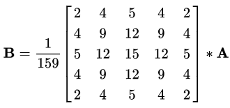
5x5高斯核,星号“*”表示卷积运算。
B.强度梯度
然后使用平滑化的图像沿x轴和y轴应用Sobel,Roberts或Prewitt内核(OpenCV中使用了Sobel),以检测边缘是水平,垂直还是对角线。(在这里你可以先不用管Sobel,Roberts或Prewitt内核,他们是什么。)
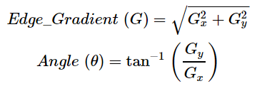
Sobel内核,用于计算水平和垂直方向的一阶导数
C.非最大抑制
非最大抑制可应用于削“薄(thin)”并有效锐化边缘。对于每个像素,检查该值是否在先前计算的渐变方向上是局部最大值。

三点非最大抑制
A在具有垂直方向的边缘上。由于梯度垂直于边缘方向,因此将B和C的像素值与A的像素值进行比较,以确定A是否为局部最大值。如果A是局部最大值,则对下一个点测试非最大值抑制;否则,将A的像素值设置为零,并抑制A。
D.磁滞阈值
在非最大抑制之后,确认强像素位于边缘的最终贴图中。但是,应进一步分析弱像素,以确定其构成为边缘还是噪声。应用两个预定义的minVal和maxVal阈值,我们设置强度梯度大于maxVal的任何像素为边缘,强度梯度小于minVal的任何像素都不为边缘并丢弃。如果亮度梯度介于minVal和maxVal之间的像素连接到强度梯度大于maxVal的像素,则仅将其视为边缘。

图1 两行磁滞阈值示例
边缘A高于maxVal,因此被视为边缘。边缘B在maxVal和minVal之间,但未连接到maxVal以上的任何边缘,因此将其丢弃。边缘C在maxVal和minVal之间,并连接到边缘A,即maxVal之上的边缘,因此被视为边缘。
对于该算法流程,我们首先要对视频帧进行灰度处理,因为我们只需要用于检测边缘的亮度通道,并应用5 x 5高斯模糊来减少噪声以减少虚假边缘。
# import cv2 as cvdef do_canny(frame):# Converts frame to grayscale because we only need the luminance channel for detecting edges - less computationally expensivegray = cv.cvtColor(frame, cv.COLOR_RGB2GRAY)# Applies a 5x5 gaussian blur with deviation of 0 to frame - not mandatory since Canny will do this for usblur = cv.GaussianBlur(gray, (5, 5), 0)# Applies Canny edge detector with minVal of 50 and maxVal of 150canny = cv.Canny(blur, 50, 150)return canny# cap = cv.VideoCapture("input.mp4")# while (cap.isOpened()):# ret, frame = cap.read()canny = do_canny(frame)# if cv.waitKey(10) & 0xFF == ord('q'):# break# cap.release()# cv.destroyAllWindows()
4.分割车道区域
我们将手工制作一个三角形的蒙版,以分割车道区域,并丢弃车架中无关的区域,以提高我们后期的效率。 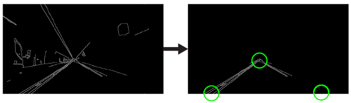 三角形遮罩将由三个坐标定义,用绿色圆圈表示。
# import cv2 as cvimport numpy as npimport matplotlib.pyplot as plt# def do_canny(frame):# gray = cv.cvtColor(frame, cv.COLOR_RGB2GRAY)# blur = cv.GaussianBlur(gray, (5, 5), 0)# canny = cv.Canny(blur, 50, 150)# return cannydef do_segment(frame):# Since an image is a multi-directional array containing the relative intensities of each pixel in the image, we can use frame.shape to return a tuple: [number of rows, number of columns, number of channels] of the dimensions of the frame# frame.shape[0] give us the number of rows of pixels the frame has. Since height begins from 0 at the top, the y-coordinate of the bottom of the frame is its heightheight = frame.shape[0]# Creates a triangular polygon for the mask defined by three (x, y) coordinatespolygons = np.array([height), (800, height), (380, 290)]])# Creates an image filled with zero intensities with the same dimensions as the framemask = np.zeros_like(frame)# Allows the mask to be filled with values of 1 and the other areas to be filled with values of 0polygons, 255)# A bitwise and operation between the mask and frame keeps only the triangular area of the framesegment = cv.bitwise_and(frame, mask)return segment# cap = cv.VideoCapture("input.mp4")# while (cap.isOpened()):# ret, frame = cap.read()# canny = do_canny(frame)# First, visualize the frame to figure out the three coordinates defining the triangular maskplt.imshow(frame)plt.show()segment = do_segment(canny)# if cv.waitKey(10) & 0xFF == ord('q'):# break# cap.release()# cv.destroyAllWindows()
5.霍夫变换
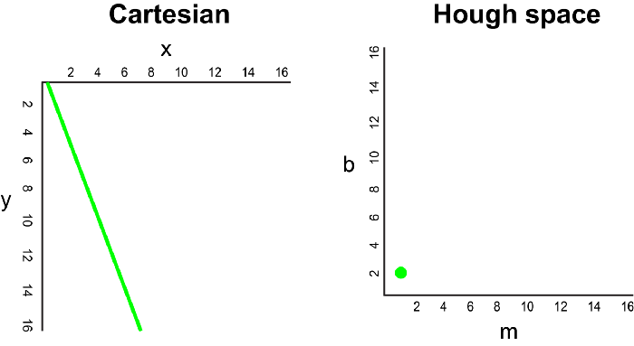
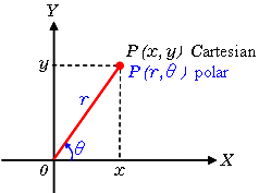
在笛卡尔坐标系中,通过将y相对于x绘制,可以将一条直线表示为y = mx + b。但是,我们也可以通过将b相对于m绘制,将该线表示为Hough Space 霍夫空间中的单个点。例如,在霍夫空间中,具有等式y = 2x +1的线可以表示为(2,1)。
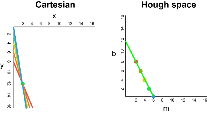
现在,如果要代替直线,我们必须在笛卡尔坐标系中绘制一个点。有许多可能的线可以通过此点,每条线的参数m和b的值均不同。例如,可以通过y = 2x + 8,y = 3x + 6,y = 4x + 4,y = 5x + 2,y = 6x来传递 (2,12) 点。这些可能的线可以在Hough空间中绘制为(2,8),(3,6),(4,4),(5,2),(6,0)。请注意,这会在Hough空间中针对b坐标生成一条m线。
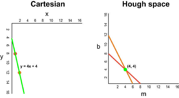
每当我们看到笛卡尔坐标系中的一系列点并且知道这些点由某条线连接时,我们就可以通过首先将笛卡尔坐标系中的每个点绘制到Hough空间中的对应线上,然后找到该线的方程。在霍夫空间中找到交点。霍夫空间中的交点表示连续通过序列中所有点的m和b值。
由于通过Canny Detector的帧可以简单地解释为代表我们图像空间中边缘的一系列白点,因此我们可以应用相同的技术来识别这些点中的哪些连接到同一条线上,以及它们是否已连接,它的等式是什么,以便我们可以在框架上绘制这条线。
为了简化说明,我们使用笛卡尔坐标来对应霍夫空间。但是,这种方法存在一个数学缺陷:当直线垂直时,渐变为无穷大,无法在霍夫空间中表示。 为了解决这个问题,我们将使用极坐标。除了在霍夫空间中将m相对于b绘制之外,该过程仍然相同,我们将r相对于θ进行绘制。
例如,对于极坐标系上x = 8和y = 6,x = 4和y = 9,x = 12和y = 3的点,我们可以绘制相应的霍夫空间。
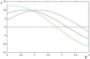
我们看到,霍夫空间中的线在θ= 0.925和r = 9.6处相交。由于极坐标系中的一条线由r =xcosθ+ysinθ给出,因此我们可以得出一条穿过所有这些点的单线定义为9.6 = xcos0.925 + ysin0.925。
通常,在霍夫空间中相交的曲线越多,意味着该相交所代表的线对应于更多的点。对于我们的实现,我们将在霍夫空间中定义一个最小阈值交叉点以检测一条线。因此,霍夫变换基本上可以跟踪帧中每个点的霍夫空间相交。如果交叉点的数量超过定义的阈值,我们将确定一条具有相应θ和r参数的线。
我们应用霍夫变换来识别两条直线,这将是我们的左右车道边界。
import cv2 as cvimport numpy as np# import matplotlib.pyplot as plt# def do_canny(frame):gray = cv.cvtColor(frame, cv.COLOR_RGB2GRAY)blur = cv.GaussianBlur(gray, (5, 5), 0)canny = cv.Canny(blur, 50, 150)return canny# def do_segment(frame):height = frame.shape[0]polygons = np.array([[(0, height), (800, height), (380, 290)]])mask = np.zeros_like(frame)cv.fillPoly(mask, polygons, 255)segment = cv.bitwise_and(frame, mask)return segment# cap = cv.VideoCapture("input.mp4")while (cap.isOpened()):ret, frame = cap.read()canny = do_canny(frame)# plt.imshow(frame)# plt.show()segment = do_segment(canny)# cv.HoughLinesP(frame, distance resolution of accumulator in pixels (larger = less precision), angle resolution of accumulator in radians (larger = less precision), threshold of minimum number of intersections, empty placeholder array, minimum length of line in pixels, maximum distance in pixels between disconnected lines)hough = cv.HoughLinesP(segment, 2, np.pi / 180, 100, np.array([]), minLineLength = 100, maxLineGap = 50)# if cv.waitKey(10) & 0xFF == ord('q'):break# cap.release()cv.destroyAllWindows()
6.可视化
车道显示为两个浅绿色,线性拟合的多项式,这些多项式将覆盖在我们的输入框中。
# import cv2 as cv# import numpy as np# # import matplotlib.pyplot as plt# def do_canny(frame):# gray = cv.cvtColor(frame, cv.COLOR_RGB2GRAY)# blur = cv.GaussianBlur(gray, (5, 5), 0)# canny = cv.Canny(blur, 50, 150)# return canny# def do_segment(frame):# height = frame.shape[0]# polygons = np.array([# [(0, height), (800, height), (380, 290)]# ])# mask = np.zeros_like(frame)# cv.fillPoly(mask, polygons, 255)# segment = cv.bitwise_and(frame, mask)# return segmentdef calculate_lines(frame, lines):# Empty arrays to store the coordinates of the left and right linesleft = []right = []# Loops through every detected linefor line in lines:# Reshapes line from 2D array to 1D arrayy1, x2, y2 = line.reshape(4)# Fits a linear polynomial to the x and y coordinates and returns a vector of coefficients which describe the slope and y-interceptparameters = np.polyfit((x1, x2), (y1, y2), 1)slope = parameters[0]y_intercept = parameters[1]# If slope is negative, the line is to the left of the lane, and otherwise, the line is to the right of the laneif slope < 0:y_intercept))else:y_intercept))# Averages out all the values for left and right into a single slope and y-intercept value for each lineleft_avg = np.average(left, axis = 0)right_avg = np.average(right, axis = 0)# Calculates the x1, y1, x2, y2 coordinates for the left and right linesleft_line = calculate_coordinates(frame, left_avg)right_line = calculate_coordinates(frame, right_avg)return np.array([left_line, right_line])def calculate_coordinates(frame, parameters):intercept = parameters# Sets initial y-coordinate as height from top down (bottom of the frame)y1 = frame.shape[0]# Sets final y-coordinate as 150 above the bottom of the framey2 = int(y1 - 150)# Sets initial x-coordinate as (y1 - b) / m since y1 = mx1 + bx1 = int((y1 - intercept) / slope)# Sets final x-coordinate as (y2 - b) / m since y2 = mx2 + bx2 = int((y2 - intercept) / slope)return np.array([x1, y1, x2, y2])def visualize_lines(frame, lines):# Creates an image filled with zero intensities with the same dimensions as the framelines_visualize = np.zeros_like(frame)# Checks if any lines are detectedif lines is not None:for x1, y1, x2, y2 in lines:# Draws lines between two coordinates with green color and 5 thickness(x1, y1), (x2, y2), (0, 255, 0), 5)return lines_visualize# cap = cv.VideoCapture("input.mp4")# while (cap.isOpened()):# ret, frame = cap.read()# canny = do_canny(frame)# # plt.imshow(frame)# # plt.show()# segment = do_segment(canny)# hough = cv.HoughLinesP(segment, 2, np.pi / 180, 100, np.array([]), minLineLength = 100, maxLineGap = 50)# Averages multiple detected lines from hough into one line for left border of lane and one line for right border of lanelines = calculate_lines(frame, hough)# Visualizes the lineslines_visualize = visualize_lines(frame, lines)# Overlays lines on frame by taking their weighted sums and adding an arbitrary scalar value of 1 as the gamma argumentoutput = cv.addWeighted(frame, 0.9, lines_visualize, 1, 1)# Opens a new window and displays the output frameoutput)# if cv.waitKey(10) & 0xFF == ord('q'):# break# cap.release()# cv.destroyAllWindows()
现在,打开Terminal并运行pythondetector.py来测试您的简单车道检测器!如果您错过任何代码,这是带有注释的完整解决方案:
import cv2 as cvimport numpy as np# import matplotlib.pyplot as pltdef do_canny(frame):# Converts frame to grayscale because we only need the luminance channel for detecting edges - less computationally expensivegray = cv.cvtColor(frame, cv.COLOR_RGB2GRAY)# Applies a 5x5 gaussian blur with deviation of 0 to frame - not mandatory since Canny will do this for usblur = cv.GaussianBlur(gray, (5, 5), 0)# Applies Canny edge detector with minVal of 50 and maxVal of 150canny = cv.Canny(blur, 50, 150)return cannydef do_segment(frame):# Since an image is a multi-directional array containing the relative intensities of each pixel in the image, we can use frame.shape to return a tuple: [number of rows, number of columns, number of channels] of the dimensions of the frame# frame.shape[0] give us the number of rows of pixels the frame has. Since height begins from 0 at the top, the y-coordinate of the bottom of the frame is its heightheight = frame.shape[0]# Creates a triangular polygon for the mask defined by three (x, y) coordinatespolygons = np.array([height), (800, height), (380, 290)]])# Creates an image filled with zero intensities with the same dimensions as the framemask = np.zeros_like(frame)# Allows the mask to be filled with values of 1 and the other areas to be filled with values of 0polygons, 255)# A bitwise and operation between the mask and frame keeps only the triangular area of the framesegment = cv.bitwise_and(frame, mask)return segmentdef calculate_lines(frame, lines):# Empty arrays to store the coordinates of the left and right linesleft = []right = []# Loops through every detected linefor line in lines:# Reshapes line from 2D array to 1D arrayy1, x2, y2 = line.reshape(4)# Fits a linear polynomial to the x and y coordinates and returns a vector of coefficients which describe the slope and y-interceptparameters = np.polyfit((x1, x2), (y1, y2), 1)slope = parameters[0]y_intercept = parameters[1]# If slope is negative, the line is to the left of the lane, and otherwise, the line is to the right of the laneif slope < 0:y_intercept))else:y_intercept))# Averages out all the values for left and right into a single slope and y-intercept value for each lineleft_avg = np.average(left, axis = 0)right_avg = np.average(right, axis = 0)# Calculates the x1, y1, x2, y2 coordinates for the left and right linesleft_line = calculate_coordinates(frame, left_avg)right_line = calculate_coordinates(frame, right_avg)return np.array([left_line, right_line])def calculate_coordinates(frame, parameters):intercept = parameters# Sets initial y-coordinate as height from top down (bottom of the frame)y1 = frame.shape[0]# Sets final y-coordinate as 150 above the bottom of the framey2 = int(y1 - 150)# Sets initial x-coordinate as (y1 - b) / m since y1 = mx1 + bx1 = int((y1 - intercept) / slope)# Sets final x-coordinate as (y2 - b) / m since y2 = mx2 + bx2 = int((y2 - intercept) / slope)return np.array([x1, y1, x2, y2])def visualize_lines(frame, lines):# Creates an image filled with zero intensities with the same dimensions as the framelines_visualize = np.zeros_like(frame)# Checks if any lines are detectedif lines is not None:for x1, y1, x2, y2 in lines:# Draws lines between two coordinates with green color and 5 thickness(x1, y1), (x2, y2), (0, 255, 0), 5)return lines_visualize# The video feed is read in as a VideoCapture objectcap = cv.VideoCapture("input.mp4")while (cap.isOpened()):# ret = a boolean return value from getting the frame, frame = the current frame being projected in the videoframe = cap.read()canny = do_canny(frame)canny)# plt.imshow(frame)# plt.show()segment = do_segment(canny)hough = cv.HoughLinesP(segment, 2, np.pi / 180, 100, np.array([]), minLineLength = 100, maxLineGap = 50)# Averages multiple detected lines from hough into one line for left border of lane and one line for right border of lanelines = calculate_lines(frame, hough)# Visualizes the lineslines_visualize = visualize_lines(frame, lines)lines_visualize)# Overlays lines on frame by taking their weighted sums and adding an arbitrary scalar value of 1 as the gamma argumentoutput = cv.addWeighted(frame, 0.9, lines_visualize, 1, 1)# Opens a new window and displays the output frameoutput)# Frames are read by intervals of 10 milliseconds. The programs breaks out of the while loop when the user presses the 'q' keyif cv.waitKey(10) & 0xFF == ord('q'):break# The following frees up resources and closes all windowscap.release()cv.destroyAllWindows()
方法2:Spatial CNN
方法1中这种相当手工制作的传统方法似乎运行得很好……至少对于清晰的直行道路而言,是的。
但是,此方法也很明显,它会在弯道或急转弯时立即中断。此外,我们注意到,由车道上的直线组成的标记(如涂上的箭头标志)的存在可能会不时使车道检测器感到困惑,这从演示渲染中的毛刺中可以明显看出。克服此问题的一种方法可能是将三角形蒙版进一步细化为两个单独的更精确的蒙版。 但是,这些相当随意的蒙版参数根本无法适应各种变化的道路环境。另一个缺点是,带点标记或根本没有清晰标记的车道也会被车道检测器忽略,因为不存在满足霍夫变换阈值的连续直线。最后,影响线路可见度的天气和照明条件也可能是一个问题。
1.Architecture
尽管卷积神经网络(CNN)已被证明是识别较低图像层的简单特征(例如边缘,颜色渐变)以及更深层次的复杂特征和实体(例如对象识别)的有效架构,但它们常常难以代表这些特征和实体的“姿势”——也就是说,CNN非常适合从原始像素中提取语义,但是在捕获帧中像素的空间关系(例如旋转和平移关系)时表现不佳。但是,这些空间关系对于车道检测任务很重要,在车道检测中,先验形状较强,而外观连贯性较弱。
例如,很难通过提取语义特征来确定交通标志,因为交通标志缺乏明显和连贯的外观提示,并且经常被遮挡。
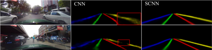
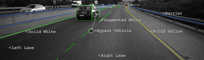
左上方图像右侧的汽车和左下方图像右侧的摩托车遮挡了右侧车道标记,并对CNN结果产生负面影响
但是,由于我们知道交通信号杆通常表现出相似的空间关系,例如垂直站立并放置在道路的左右两侧,因此我们看到了增强空间信息的重要性。接下来是检测车道的类似情况。
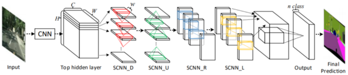
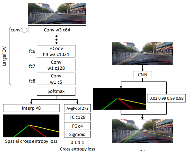
为了解决这个问题,Xingang Pan, Jianping Shi等人提出了一种架构Spatial CNN(SCNN),“将传统的深层逐层卷积概括为特征图中的逐层卷积”。这是什么意思?在传统的逐层CNN中,每个卷积层都从其前一层接收输入,进行卷积和非线性激活,然后将输出发送到下一层。SCNN通过将各个要素地图的行和列视为“层”,进一步采取了这一步骤,并依次应用了相同的过程(其中顺序表示切片仅在从先前切片接收到信息之后才将信息传递给后续切片),允许像素信息在同一层内的神经元之间传递消息,从而有效地增加了对空间信息的重视。
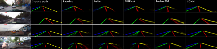
SCNN还相对较新,发布于2018年,但已经跑赢了ReNet(RNN),MRFNet(MRF + CNN),更深入的ResNet架构之类,并以96.53% 的准确性在TuSimple基准测试车道检测挑战赛中排名第一。
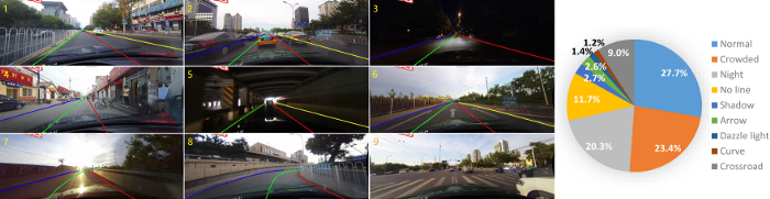
此外,除了SCNN的发布之外,作者还发布了CULane Dataset,这是一个大规模数据集,带有带有立方棘刺的行车道注释。CULane数据集还包含许多具有挑战性的场景,包括遮挡和变化的照明条件。
2.模型
车道检测需要精确的像素识别和车道曲线预测。SCNN的作者没有直接训练车道的存在并随后进行聚类,而是将蓝色,绿色,红色和黄色的车道标记视为四个单独的类。该模型为每个曲线输出概率图(概率图),类似于语义分割任务,然后将概率图通过一个小型网络传递,以预测最终的立方棘。该模型基于DeepLab-LargeFOV模型变体。
GitHub 链接 | https://github.com/XingangPan/SCNN
对于存在值超过0.5的每个车道标记,将以20行间隔搜索对应的概率图,以找到响应度最高的位置。为了确定是否检测到车道标记,计算地面真相(正确标签)和预测之间的“联合路口”(IoU),其中将高于设置阈值的IoU评估为“真阳性”(TP),以计算精度和记起。
3.测试和训练
全部代码已经上传至Github上,您可以按照此仓库在SCNN论文中重现结果,或使用CULane数据集测试您自己的模型。
👉 车道线检测项目论文和数据集 https://github.com/Charmve/Awesome-Lane-Detection
总结
就是这样!🎉希望本教程向您展示了如何使用涉及许多手工功能和微调的传统方法来构建简单的车道检测器,并且还向您介绍了一种替代方法,该方法遵循了解决几乎所有类型的车辆的最新趋势。计算机视觉问题:您可以为此添加卷积神经网络!
更多精彩学习资料,承诺大家的,一个也不会少,我分类整理好并附上链接。
GitHub上开源:https://github.com/Charmve/computer-vision-in-action
往期精彩回顾
本站qq群851320808,加入微信群请扫码: