
高斯朴素贝叶斯分类的原理解释和手写代码实现

来源:DeepHub IMBA 本文约3500字,建议阅读10+分钟
本文与你介绍高斯分布的基本概念及代码实现。
什么是高斯分布?
多分类的高斯朴素贝叶斯
from random import randomfrom random import randintimport pandas as pdimport numpy as npimport seaborn as snsimport matplotlib.pyplot as pltimport statisticsfrom sklearn.model_selection import train_test_splitfrom sklearn.preprocessing import StandardScalerfrom sklearn.naive_bayes import GaussianNBfrom sklearn.metrics import confusion_matrixfrom mlxtend.plotting import plot_decision_regions
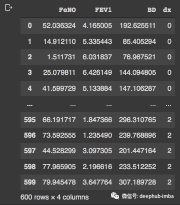
#Creating values for FeNO with 3 classes:FeNO_0 = np.random.normal(20, 19, 200)FeNO_1 = np.random.normal(40, 20, 200)FeNO_2 = np.random.normal(60, 20, 200)#Creating values for FEV1 with 3 classes:FEV1_0 = np.random.normal(4.65, 1, 200)FEV1_1 = np.random.normal(3.75, 1.2, 200)FEV1_2 = np.random.normal(2.85, 1.2, 200)#Creating values for Broncho Dilation with 3 classes:BD_0 = np.random.normal(150,49, 200)BD_1 = np.random.normal(201,50, 200)BD_2 = np.random.normal(251, 50, 200)#Creating labels variable with three classes:(2)disease (1)possible disease (0)no disease:not_asthma = np.zeros((200,), dtype=int)poss_asthma = np.ones((200,), dtype=int)asthma = np.full((200,), 2, dtype=int)#Concatenate classes into one variable:FeNO = np.concatenate([FeNO_0, FeNO_1, FeNO_2])FEV1 = np.concatenate([FEV1_0, FEV1_1, FEV1_2])BD = np.concatenate([BD_0, BD_1, BD_2])dx = np.concatenate([not_asthma, poss_asthma, asthma])#Create DataFrame:df = pd.DataFrame()#Add variables to DataFrame:df['FeNO'] = FeNO.tolist()df['FEV1'] = FEV1.tolist()df['BD'] = BD.tolist()df['dx'] = dx.tolist()#Check database:df
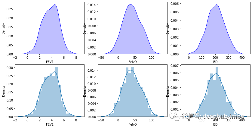
fig, axs = plt.subplots(2, 3, figsize=(14, 7))sns.kdeplot(df['FEV1'], shade=True, color="b", ax=axs[0, 0])sns.kdeplot(df['FeNO'], shade=True, color="b", ax=axs[0, 1])sns.kdeplot(df['BD'], shade=True, color="b", ax=axs[0, 2])sns.distplot( a=df["FEV1"], hist=True, kde=True, rug=False, ax=axs[1, 0])sns.distplot( a=df["FeNO"], hist=True, kde=True, rug=False, ax=axs[1, 1])sns.distplot( a=df["BD"], hist=True, kde=True, rug=False, ax=axs[1, 2])plt.show()
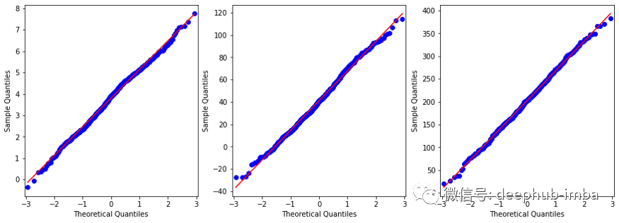
from statsmodels.graphics.gofplots import qqplotfrom matplotlib import pyplot#q-q plot:fig, axs = pyplot.subplots(1, 3, figsize=(15, 5))qqplot(df['FEV1'], line='s', ax=axs[0])qqplot(df['FeNO'], line='s', ax=axs[1])qqplot(df['BD'], line='s', ax=axs[2])pyplot.show()
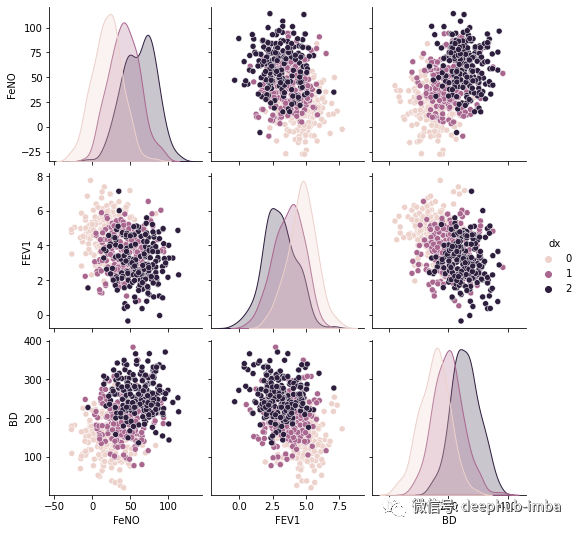
#Exploring dataset:sns.pairplot(df, kind="scatter", hue="dx")plt.show()
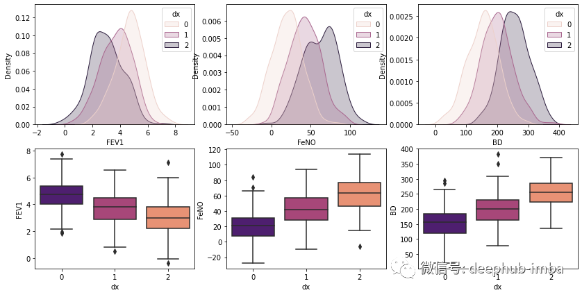
# plotting both distibutions on the same figurefig, axs = plt.subplots(2, 3, figsize=(14, 7))fig = sns.kdeplot(df['FEV1'], hue= df['dx'], shade=True, color="r", ax=axs[0, 0])fig = sns.kdeplot(df['FeNO'], hue= df['dx'], shade=True, color="r", ax=axs[0, 1])fig = sns.kdeplot(df['BD'], hue= df['dx'], shade=True, color="r", ax=axs[0, 2])sns.boxplot(x=df["dx"], y=df["FEV1"], palette = 'magma', ax=axs[1, 0])sns.boxplot(x=df["dx"], y=df["FeNO"], palette = 'magma',ax=axs[1, 1])sns.boxplot(x=df["dx"], y=df["BD"], palette = 'magma',ax=axs[1, 2])plt.show()
手写朴素贝叶斯分类
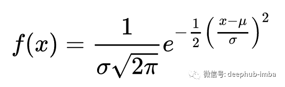
def normal_dist(x , mean , sd):prob_density = (1/sd*np.sqrt(2*np.pi)) * np.exp(-0.5*((x-mean)/sd)**2)return prob_density
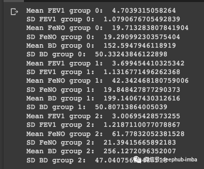
#Group 0:group_0 = df[df['dx'] == 0]print('Mean FEV1 group 0: ', statistics.mean(group_0['FEV1']))print('SD FEV1 group 0: ', statistics.stdev(group_0['FEV1']))print('Mean FeNO group 0: ', statistics.mean(group_0['FeNO']))print('SD FeNO group 0: ', statistics.stdev(group_0['FeNO']))print('Mean BD group 0: ', statistics.mean(group_0['BD']))print('SD BD group 0: ', statistics.stdev(group_0['BD']))#Group 1:group_1 = df[df['dx'] == 1]print('Mean FEV1 group 1: ', statistics.mean(group_1['FEV1']))print('SD FEV1 group 1: ', statistics.stdev(group_1['FEV1']))print('Mean FeNO group 1: ', statistics.mean(group_1['FeNO']))print('SD FeNO group 1: ', statistics.stdev(group_1['FeNO']))print('Mean BD group 1: ', statistics.mean(group_1['BD']))print('SD BD group 1: ', statistics.stdev(group_1['BD']))#Group 2:group_2 = df[df['dx'] == 2]print('Mean FEV1 group 2: ', statistics.mean(group_2['FEV1']))print('SD FEV1 group 2: ', statistics.stdev(group_2['FEV1']))print('Mean FeNO group 2: ', statistics.mean(group_2['FeNO']))print('SD FeNO group 2: ', statistics.stdev(group_2['FeNO']))print('Mean BD group 2: ', statistics.mean(group_2['BD']))print('SD BD group 2: ', statistics.stdev(group_2['BD']))
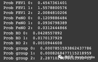
#Probability for:#FEV1 = 2.75#FeNO = 27#BD = 125#We have the same number of observations, so the general probability is: 0.33Prob_geral = round(0.333, 3)#Prob FEV1:Prob_FEV1_0 = round(normal_dist(2.75, 4.70, 1.08), 10)print('Prob FEV1 0: ', Prob_FEV1_0)Prob_FEV1_1 = round(normal_dist(2.75, 3.70, 1.13), 10)print('Prob FEV1 1: ', Prob_FEV1_1)Prob_FEV1_2 = round(normal_dist(2.75, 3.01, 1.22), 10)print('Prob FEV1 2: ', Prob_FEV1_2)#Prob FeNO:Prob_FeNO_0 = round(normal_dist(27, 19.71, 19.29), 10)print('Prob FeNO 0: ', Prob_FeNO_0)Prob_FeNO_1 = round(normal_dist(27, 42.34, 19.85), 10)print('Prob FeNO 1: ', Prob_FeNO_1)Prob_FeNO_2 = round(normal_dist(27, 61.78, 21.39), 10)print('Prob FeNO 2: ', Prob_FeNO_2)#Prob BD:Prob_BD_0 = round(normal_dist(125, 152.59, 50.33), 10)print('Prob BD 0: ', Prob_BD_0)Prob_BD_1 = round(normal_dist(125, 199.14, 50.81), 10)print('Prob BD 1: ', Prob_BD_1)Prob_BD_2 = round(normal_dist(125, 256.13, 47.04), 10)print('Prob BD 2: ', Prob_BD_2)#Compute probability:Prob_group_0 = Prob_geral*Prob_FEV1_0*Prob_FeNO_0*Prob_BD_0print('Prob group 0: ', Prob_group_0)Prob_group_1 = Prob_geral*Prob_FEV1_1*Prob_FeNO_1*Prob_BD_1print('Prob group 1: ', Prob_group_1)Prob_group_2 = Prob_geral*Prob_FEV1_2*Prob_FeNO_2*Prob_BD_2print('Prob group 2: ', Prob_group_2)
Scikit-Learn的分类器样例
#Creating X and y:X = df.drop('dx', axis=1)y = df['dx']#Data split into train and test:X_train, X_test, y_train, y_test = train_test_split(X, y, test_size=0.30)
sc = StandardScaler()X_train = sc.fit_transform(X_train)X_test = sc.transform(X_test)
#Build the model:classifier = GaussianNB()classifier.fit(X_train, y_train)#Evaluate the model:print("training set score: %f" % classifier.score(X_train, y_train))print("test set score: %f" % classifier.score(X_test, y_test))
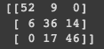
# Predicting the Test set resultsy_pred = classifier.predict(X_test)#Confusion Matrix:cm = confusion_matrix(y_test, y_pred)print(cm)
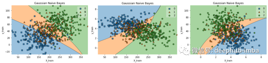
df.to_csv('data.csv', index = False)data = pd.read_csv('data.csv')def gaussian_nb_a(data):x = data[['BD','FeNO',]].valuesy = data['dx'].astype(int).valuesGauss_nb = GaussianNB()Gauss_nb.fit(x,y)print(Gauss_nb.score(x,y))#Plot decision region:plot_decision_regions(x,y, clf=Gauss_nb, legend=1)#Adding axes annotations:plt.xlabel('X_train')plt.ylabel('y_train')plt.title('Gaussian Naive Bayes')plt.show()def gaussian_nb_b(data):x = data[['BD','FEV1',]].valuesy = data['dx'].astype(int).valuesGauss_nb = GaussianNB()Gauss_nb.fit(x,y)print(Gauss_nb.score(x,y))#Plot decision region:plot_decision_regions(x,y, clf=Gauss_nb, legend=1)#Adding axes annotations:plt.xlabel('X_train')plt.ylabel('y_train')plt.title('Gaussian Naive Bayes')plt.show()def gaussian_nb_c(data):x = data[['FEV1','FeNO',]].valuesy = data['dx'].astype(int).valuesGauss_nb = GaussianNB()Gauss_nb.fit(x,y)print(Gauss_nb.score(x,y))#Plot decision region:plot_decision_regions(x,y, clf=Gauss_nb, legend=1)#Adding axes annotations:plt.xlabel('X_train')plt.ylabel('y_train')plt.title('Gaussian Naive Bayes')plt.show()gaussian_nb_a(data)gaussian_nb_b(data)gaussian_nb_c(data)
评论