
图异常点检测算法OddBall(附代码)
大家好,我是爱生活,AI风控的小伍哥,上次给大家带来第一篇文章OddBall,当时并未附代码,现在找到一个比较好的开源代码,分享给大家。
项目地址:https://github.com/gloooryyt/oddball_py3
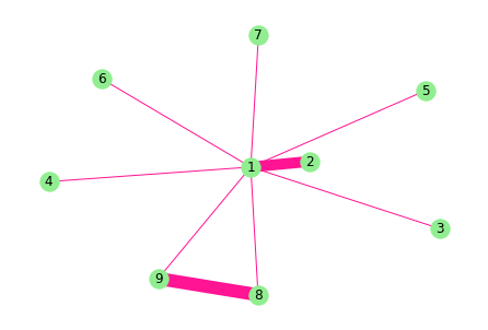
我们自己构建测试数据或者读取测试数据
import networkx as nxG = nx.Graph(date="10.11",name="无向图")#创建空图,无向图G.add_node(1)G.add_nodes_from([1,2,3,4,5,6,7,8,9])G.nodes()G.add_weighted_edges_from([(1,2,10),(1,3,1),(1,4,1),(1,5,1),(1,6,1),(1,7,1),(1,8,1),(1,9,1),(8,9,1)])print(G.adj){1: {2: {'weight': 10}, 3: {'weight': 1}, 4: {'weight': 1}, 5: {'weight': 1}, 6: {'weight': 1}, 7: {'weight': 1}, 8: {'weight': 1}, 9: {'weight': 1}}, 2: {1: {'weight': 10}}, 3: {1: {'weight': 1}}, 4: {1: {'weight': 1}}, 5: {1: {'weight': 1}}, 6: {1: {'weight': 1}}, 7: {1: {'weight': 1}}, 8: {1: {'weight': 1}, 9: {'weight': 1}}, 9: {1: {'weight': 1}, 8: {'weight': 1}}}import matplotlib.pyplot as pltedgewidth = [10,1,1,1,1,1,1,1,12]nx.draw(G,with_labels=True,pos=nx.spring_layout(G),width=edgewidth,node_color="lightgreen",edge_color="DeepPink")plt.show()
也可以读取自己的数据集
#数据读取import ospath = '/Users/wuzhengxiang/Downloads/OddBall10_tbox 2/oddball-edges.txt'
import numpy as npimport networkx as nx#load data, a weighted undirected graphdef load_data(path):data = np.loadtxt(path).astype('int32')G = nx.Graph()for ite in data:G.add_edge(ite[0], ite[1], weight=ite[2])return Gdef get_feature(G):#feature dictionary which format is {node i's id:Ni, Ei, Wi, λw,i}featureDict = {}nodelist = list(G.nodes)for ite in nodelist:featureDict[ite] = []#the number of node i's neighborNi = G.degree(ite)featureDict[ite].append(Ni)#the set of node i's neighboriNeighbor = list(G.neighbors(ite))#the number of edges in egonet iEi = 0#sum of weights in egonet iWi = 0#the principal eigenvalue(the maximum eigenvalue with abs) of egonet i's weighted adjacency matrixLambda_w_i = 0Ei += Niegonet = nx.Graph()for nei in iNeighbor:Wi += G[nei][ite]['weight']egonet.add_edge(ite, nei, weight=G[nei][ite]['weight'])iNeighborLen = len(iNeighbor)for it1 in range(iNeighborLen):for it2 in range(it1+1, iNeighborLen):#if it1 in it2's neighbor listif iNeighbor[it1] in list(G.neighbors(iNeighbor[it2])):Ei += 1Wi += G[iNeighbor[it1]][iNeighbor[it2]]['weight']egonet.add_edge(iNeighbor[it1], iNeighbor[it2], weight=G[iNeighbor[it1]][iNeighbor[it2]]['weight'])egonet_adjacency_matrix = nx.adjacency_matrix(egonet).todense()eigenvalue, eigenvector = np.linalg.eig(egonet_adjacency_matrix)eigenvalue.sort()Lambda_w_i = max(abs(eigenvalue[0]), abs(eigenvalue[-1]))featureDict[ite].append(Ei)featureDict[ite].append(Wi)featureDict[ite].append(Lambda_w_i)return featureDict
import numpy as npfrom sklearn.linear_model import LinearRegressionfrom sklearn.neighbors import LocalOutlierFactor# feature dictionary which format is {node i's id:Ni, Ei, Wi, λw,i}def star_or_clique(featureDict):N = []E = []for key in featureDict.keys():N.append(featureDict[key][0])E.append(featureDict[key][1])#E=CN^α => log on both sides => logE=logC+αlogN#regard as y=b+wx to do linear regression#here the base of log is 2y_train = np.log2(E)y_train = np.array(y_train)y_train = y_train.reshape(len(E), 1)x_train = np.log2(N)x_train = np.array(x_train)x_train = x_train.reshape(len(N), 1)model = LinearRegression()y_train)w = model.coef_[0][0]b = model.intercept_[0]C = 2**balpha = woutlineScoreDict = {}for key in featureDict.keys():yi = featureDict[key][1]xi = featureDict[key][0]outlineScore = (max(yi, C*(xi**alpha))/min(yi, C*(xi**alpha)))*np.log(abs(yi-C*(xi**alpha))+1)= outlineScorereturn outlineScoreDictdef heavy_vicinity(featureDict):W = []E = []for key in featureDict.keys():W.append(featureDict[key][2])E.append(featureDict[key][1])#W=CE^β => log on both sides => logW=logC+βlogE#regard as y=b+wx to do linear regression#here the base of log is 2y_train = np.log2(W)y_train = np.array(y_train)y_train = y_train.reshape(len(W), 1)x_train = np.log2(E)x_train = np.array(x_train)x_train = x_train.reshape(len(E), 1)model = LinearRegression()y_train)w = model.coef_[0][0]b = model.intercept_[0]C = 2**bbeta = woutlineScoreDict = {}for key in featureDict.keys():yi = featureDict[key][2]xi = featureDict[key][1]outlineScore = (max(yi, C*(xi**beta))/min(yi, C*(xi**beta)))*np.log(abs(yi-C*(xi**beta))+1)= outlineScorereturn outlineScoreDictdef dominant_edge(featureDict):Lambda_w_i = []W = []for key in featureDict.keys():Lambda_w_i.append(featureDict[key][3])W.append(featureDict[key][2])#λ=CW^γ => log on both sides => logλ=logC+γlogW#regard as y=b+wx to do linear regression#here the base of log is 2y_train = np.log2(Lambda_w_i)y_train = np.array(y_train)y_train = y_train.reshape(len(Lambda_w_i), 1)x_train = np.log2(W)x_train = np.array(x_train)x_train = x_train.reshape(len(W), 1)model = LinearRegression()y_train)w = model.coef_[0][0]b = model.intercept_[0]C = 2 ** bbeta = woutlineScoreDict = {}for key in featureDict.keys():yi = featureDict[key][3]xi = featureDict[key][2]outlineScore = (max(yi, C * (xi ** beta)) / min(yi, C * (xi ** beta))) * np.log(abs(yi - C * (xi ** beta)) + 1)= outlineScorereturn outlineScoreDictdef star_or_clique_withLOF(featureDict):N = []E = []for key in featureDict.keys():N.append(featureDict[key][0])E.append(featureDict[key][1])#E=CN^α => log on both sides => logE=logC+αlogN#regard as y=b+wx to do linear regression#here the base of log is 2y_train = np.log2(E)y_train = np.array(y_train)y_train = y_train.reshape(len(E), 1)x_train = np.log2(N)x_train = np.array(x_train)x_train = x_train.reshape(len(N), 1) #the order in x_train and y_train is the same as which in featureDict.keys() now#prepare data for LOFxAndyForLOF = []for index in range(len(N)):tempArray = np.array([x_train[index][0], y_train[index][0]])xAndyForLOF.append(tempArray)xAndyForLOF = np.array(xAndyForLOF)model = LinearRegression()y_train)w = model.coef_[0][0]b = model.intercept_[0]C = 2**balpha = w={}'.format(alpha))#LOF algorithmclf = LocalOutlierFactor(n_neighbors=20)clf.fit(xAndyForLOF)LOFScoreArray = -clf.negative_outlier_factor_outScoreDict = {}count = 0 #Used to take LOFScore in sequence from LOFScoreArray#get the maximum outLinemaxOutLine = 0for key in featureDict.keys():yi = featureDict[key][1]xi = featureDict[key][0]outlineScore = (max(yi, C*(xi**alpha))/min(yi, C*(xi**alpha)))*np.log(abs(yi-C*(xi**alpha))+1)if outlineScore > maxOutLine:maxOutLine = outlineScore={}'.format(maxOutLine))#get the maximum LOFScoremaxLOFScore = 0for ite in range(len(N)):if LOFScoreArray[ite] > maxLOFScore:maxLOFScore = LOFScoreArray[ite]={}'.format(maxLOFScore))for key in featureDict.keys():yi = featureDict[key][1]xi = featureDict[key][0]outlineScore = (max(yi, C*(xi**alpha))/min(yi, C*(xi**alpha)))*np.log(abs(yi-C*(xi**alpha))+1)LOFScore = LOFScoreArray[count]count += 1outScore = outlineScore/maxOutLine + LOFScore/maxLOFScore= outScorereturn outScoreDictdef heavy_vicinity_withLOF(featureDict):W = []E = []for key in featureDict.keys():W.append(featureDict[key][2])E.append(featureDict[key][1])#W=CE^β => log on both sides => logW=logC+βlogE#regard as y=b+wx to do linear regression#here the base of log is 2y_train = np.log2(W)y_train = np.array(y_train)y_train = y_train.reshape(len(W), 1)x_train = np.log2(E)x_train = np.array(x_train)x_train = x_train.reshape(len(E), 1) #the order in x_train and y_train is the same as which in featureDict.keys() now#prepare data for LOFxAndyForLOF = []for index in range(len(W)):tempArray = np.array([x_train[index][0], y_train[index][0]])xAndyForLOF.append(tempArray)xAndyForLOF = np.array(xAndyForLOF)model = LinearRegression()y_train)w = model.coef_[0][0]b = model.intercept_[0]C = 2**bbeta = w={}'.format(beta))#LOF algorithmclf = LocalOutlierFactor(n_neighbors=20)clf.fit(xAndyForLOF)LOFScoreArray = -clf.negative_outlier_factor_outScoreDict = {}count = 0 #Used to take LOFScore in sequence from LOFScoreArray#get the maximum outLinemaxOutLine = 0for key in featureDict.keys():yi = featureDict[key][2]xi = featureDict[key][1]outlineScore = (max(yi, C*(xi**beta))/min(yi, C*(xi**beta)))*np.log(abs(yi-C*(xi**beta))+1)if outlineScore > maxOutLine:maxOutLine = outlineScore={}'.format(maxOutLine))#get the maximum LOFScoremaxLOFScore = 0for ite in range(len(W)):if LOFScoreArray[ite] > maxLOFScore:maxLOFScore = LOFScoreArray[ite]={}'.format(maxLOFScore))for key in featureDict.keys():yi = featureDict[key][2]xi = featureDict[key][1]outlineScore = (max(yi, C*(xi**beta))/min(yi, C*(xi**beta)))*np.log(abs(yi-C*(xi**beta))+1)LOFScore = LOFScoreArray[count]count += 1outScore = outlineScore/maxOutLine + LOFScore/maxLOFScore= outScorereturn outScoreDictdef dominant_edge_withLOF(featureDict):Lambda_w_i = []W = []for key in featureDict.keys():Lambda_w_i.append(featureDict[key][3])W.append(featureDict[key][2])#λ=CW^γ => log on both sides => logλ=logC+γlogW#regard as y=b+wx to do linear regression#here the base of log is 2y_train = np.log2(Lambda_w_i)y_train = np.array(y_train)y_train = y_train.reshape(len(Lambda_w_i), 1)x_train = np.log2(W)x_train = np.array(x_train)x_train = x_train.reshape(len(W), 1) #the order in x_train and y_train is the same as which in featureDict.keys() now#prepare data for LOFxAndyForLOF = []for index in range(len(W)):tempArray = np.array([x_train[index][0], y_train[index][0]])xAndyForLOF.append(tempArray)xAndyForLOF = np.array(xAndyForLOF)model = LinearRegression()y_train)w = model.coef_[0][0]b = model.intercept_[0]C = 2**bgamma = w={}'.format(gamma))#LOF algorithmclf = LocalOutlierFactor(n_neighbors=20)clf.fit(xAndyForLOF)LOFScoreArray = -clf.negative_outlier_factor_outScoreDict = {}count = 0 #Used to take LOFScore in sequence from LOFScoreArray#get the maximum outLinemaxOutLine = 0for key in featureDict.keys():yi = featureDict[key][3]xi = featureDict[key][2]outlineScore = (max(yi, C*(xi**gamma))/min(yi, C*(xi**gamma)))*np.log(abs(yi-C*(xi**gamma))+1)if outlineScore > maxOutLine:maxOutLine = outlineScore={}'.format(maxOutLine))#get the maximum LOFScoremaxLOFScore = 0for ite in range(len(W)):if LOFScoreArray[ite] > maxLOFScore:maxLOFScore = LOFScoreArray[ite]={}'.format(maxLOFScore))for key in featureDict.keys():yi = featureDict[key][3]xi = featureDict[key][2]outlineScore = (max(yi, C*(xi**gamma))/min(yi, C*(xi**gamma)))*np.log(abs(yi-C*(xi**gamma))+1)LOFScore = LOFScoreArray[count]count += 1outScore = outlineScore/maxOutLine + LOFScore/maxLOFScore= outScorereturn outScoreDict
一、概 述
基于图的异常检测分为 孤立点检测 和 异常群簇检测,本文是孤立点检测中较经典的论文,通过研究Ego-net总结几种异常模型及提供度量方式:
异常结构 | 含义 | 度量方式 |
CliqueStar | 呈星状或者团状结构 | 边数~节点邻居数 |
HeavyVicinity | 总边权重异常大 | 总边权重~边数 |
DominantPair | 存在某条权重异常大的边 | 主特征值~总边权重 |
文章调查了Ego-net中存在的异常模式,并给出了检测异常模式的依据基于上述模式,提出了OddBall,一种用于异常点检测的无监督方法,将OddBall应用于真实数据集,并验证了算法的有效性
论文名称:OddBall: Spotting Anomalies in Weighted Graphs
论文地址:http://www.cs.cmu.edu/~mmcgloho/pubs/pakdd10.pdf
代码地址:https://www.andrew.cmu.edu/user/lakoglu/pubs.html#code
二、Ego-net(中心节点)
以中心节点(ego)及其邻居组成的子图,一般用于研究个体性质以及局部社区发现,本文仅考虑一阶邻居,这是为了减少计算量并提和高可解释性。
三、Ego-net模式及度量方法
1 、CliqueStar(基于密度)
基于密度的方法可以识别出下面两种Ego-net的异常结构:
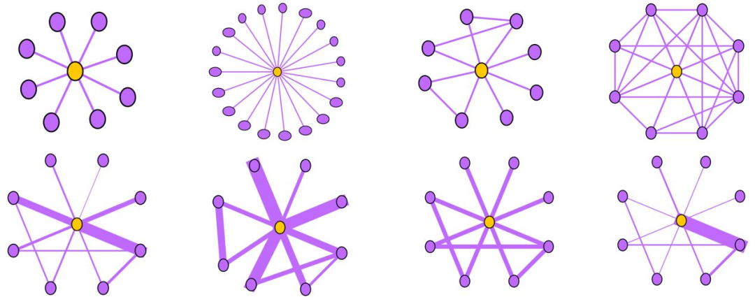
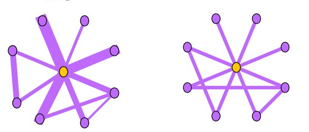
Near-Star:在正常的社交网络中,我们通常认为朋友之间可能会相互认识,因此一阶Ego-net中的邻居之间没有任何关联是非常可疑的,近似星型,邻居之间很少联系(如通话关系网络中的中介、电催人员、营销号码,他们大量的联系别人,然而联系人中之间几乎没啥联系),这种结构的Ego-net被称为star,如下图所示,中心节点与大量节点存在关联,但是邻居之间无联系或者联系很少。
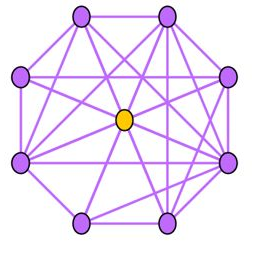
Near-Clique:与上述相反,邻居之间存在大量关联也是非常可疑的,这种结构的Ego-net被称为cliques。正如下图所示,中心节点与大量节点存在关联,邻居之间的联系非常密集,近似环状,邻居之间联系紧密(如某个讨论组、恐怖组织)。
度量方法:边数~邻居数
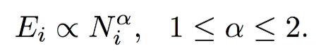
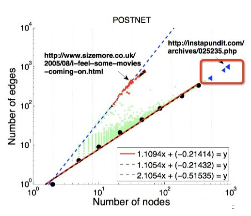
如下图所示,可以看出大多数节点Ego-net中边数 E 与邻居数 N 服从幂律分布(对数坐标后呈线性)、给定某节点i对应的 Ei 、Ni ,求出幂律系数 α ,若:
α 接近1(黑色虚线),节点i的Ego-net呈现Near-Clique
α 接近2(蓝色虚线),节点i的Ego-net呈现Near-Star
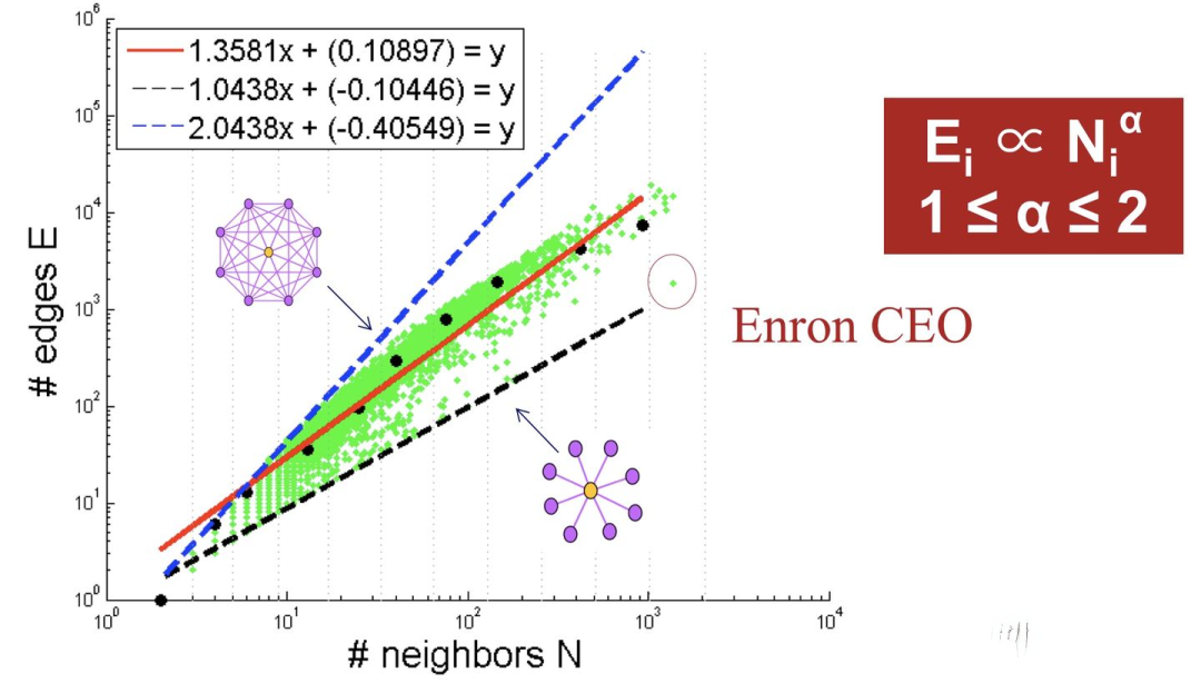 红线是拟合中位数,蓝色和黑色虚线是边界线。
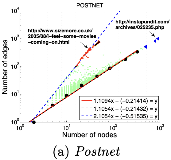
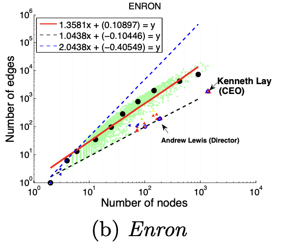
大多数Graph都遵循该模式:
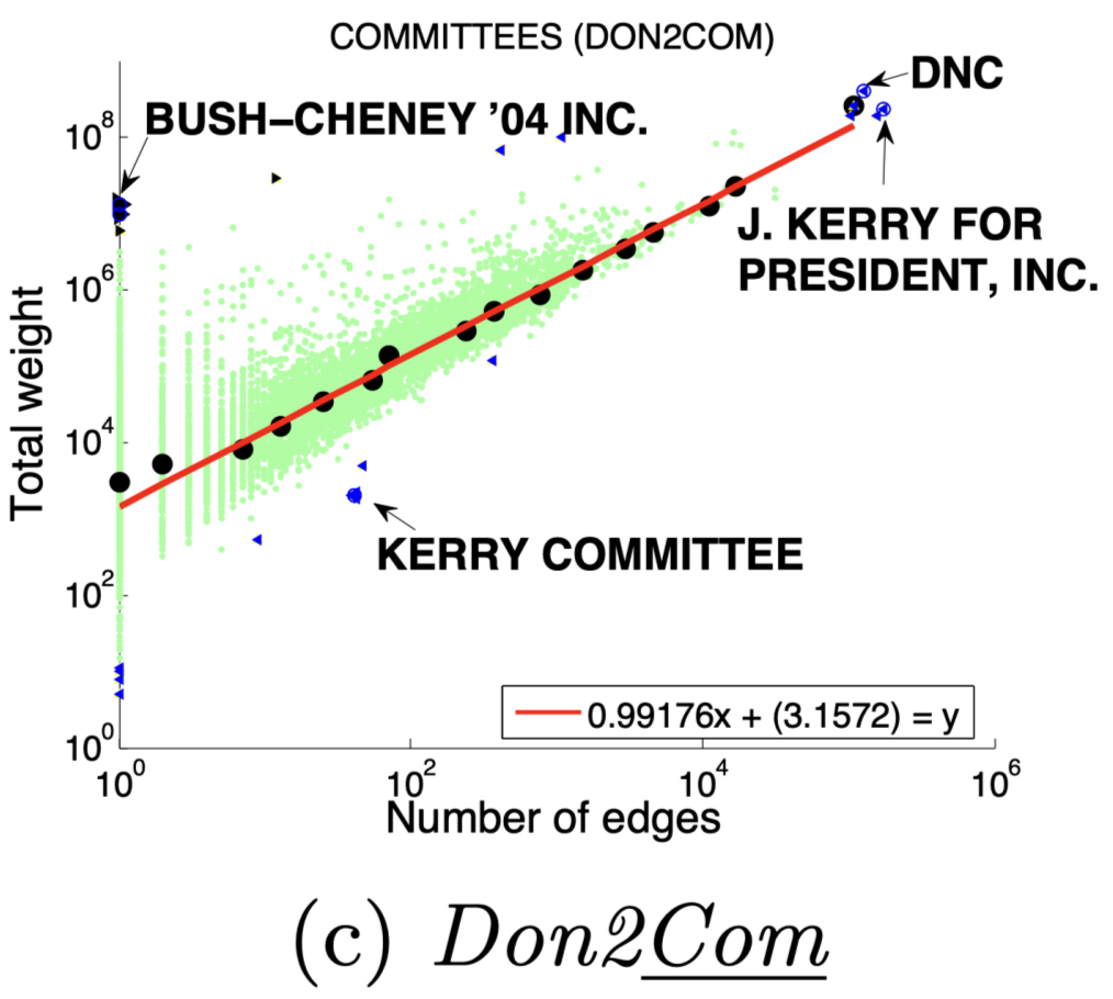
2、HeavyVicinity(权重)
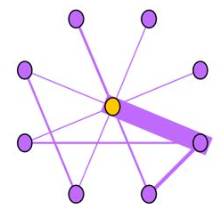
HeavyVicinity指“较重的邻居“,Ego-net中边数一定时,总边权重异常大(如骗贷者通过频繁拨打电话伪造通话记录),中心节点与一小部分节点之间存在权重非常大的关联也是可疑的,如骗贷者通过频繁拨打电话伪造通话记录。正如下图所示,中心节点与少部分节点之间的连接权重非常大。
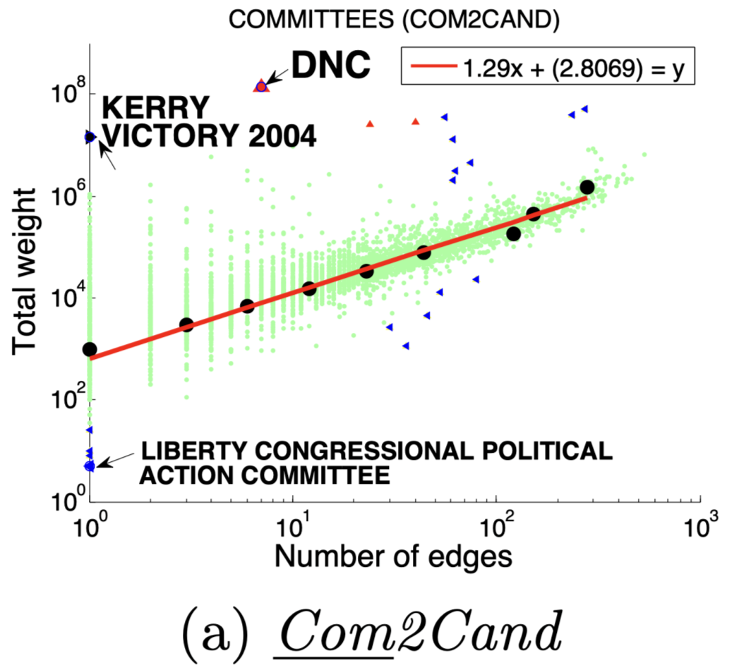
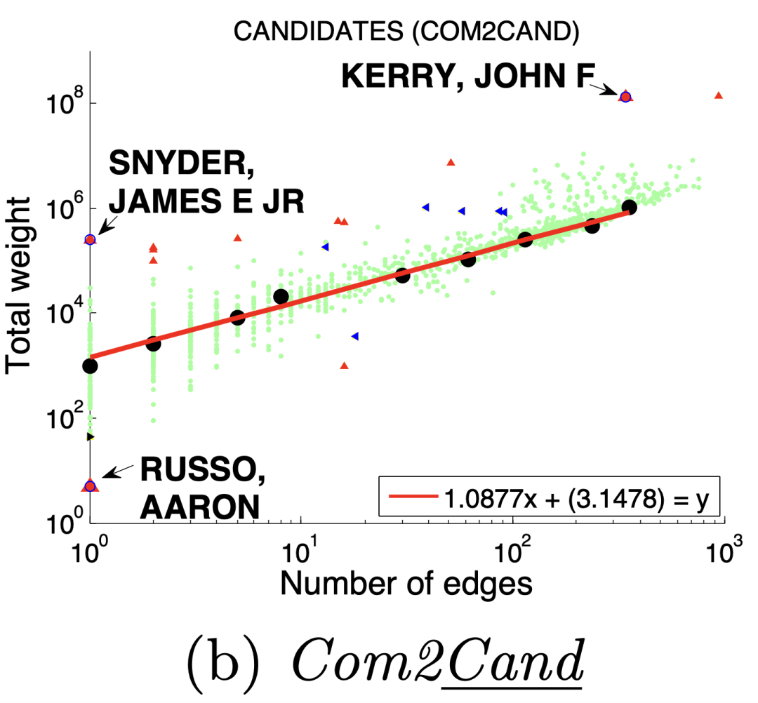
度量方法:总边权重~边数
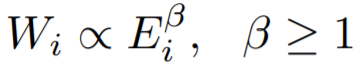
大多数节点Ego-net中总边权重~边数也服从幂律分布(对数坐标), β 越高表示越异常
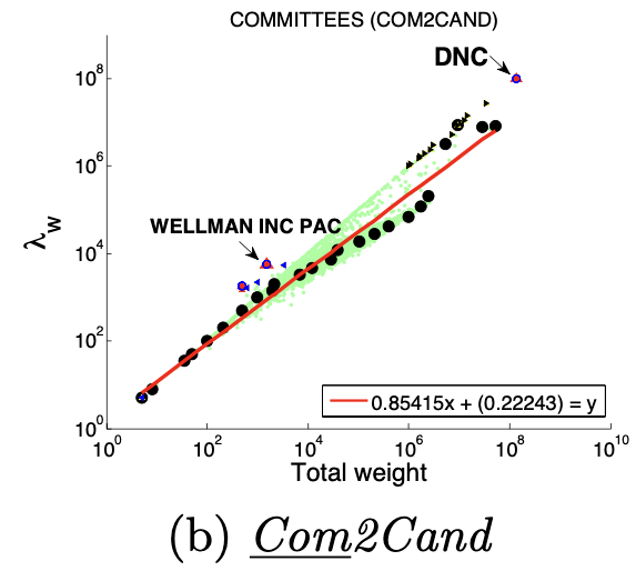
图(a)选举中,民主党(DNC)的大量的资金给为数不多的候选者
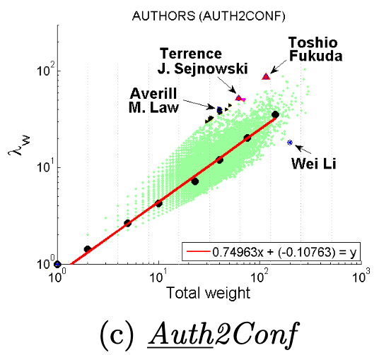
3 、DominantPair(主导边)
Dominant heavy links指“主导的边”,Ego-Net中存在某条边权重异常大(如学者投稿会议网络中,“Toshio Fukuda” 拥有115篇papers,投稿了17个会议,但其中87篇pager投稿了一个ICRA):
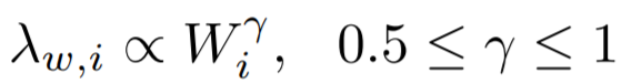
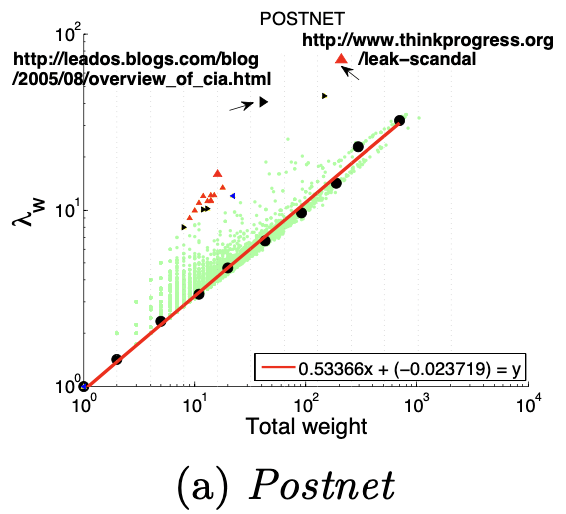
度量方法:主特征值~总权重
大多数节点Ego-net对应带权邻接矩阵中主特征值(principal eigenvalue,即最大特征值)~总边权重也服从幂律分布,其中系数 λ 表示Ego-net中边权均匀分布, λ 接近1表示存在DominantPair的情况。
四、OddBall异常检测算法
OddBall由out-line(i)和out-lof(i)两部分组成:
out-line:计算实际点与拟合直线(红线)的偏离程度。
out-lof:但out-line但会存在“缺陷是无法识别离正常点很远,但与拟合直线很近的异常点”的缺陷,故结合传统基于密度的方法LOF(也可以选其他的)。
二者集成方式先求出两个score,然后归一化(除以最大值)后求和:
out-score(i)=out-line(i)+out-lof(i)
1、out-line
 为实际值,
为实际值, 为在拟合直线(正常点)上的预测值,二者相减为偏离程度/异常程度取
log是为了平滑
 为惩罚系数:实际值偏离正常的倍数
2、out-lof
outline的缺陷:无法识别红框内的节点,故引入LOF,详情可参考:https://zhuanlan.zhihu.com/p/28178476
五、相关思考
本文中仅考虑了节点的一阶子图,将子图范围扩展到二阶或者是更大的局部子图是否会效果更好?检测模式依赖的特征是否具有鲁棒性?