ROC和AUC也不是评估机器学习性能的金标准

共 8047字，需浏览 17分钟

· 2021-06-23

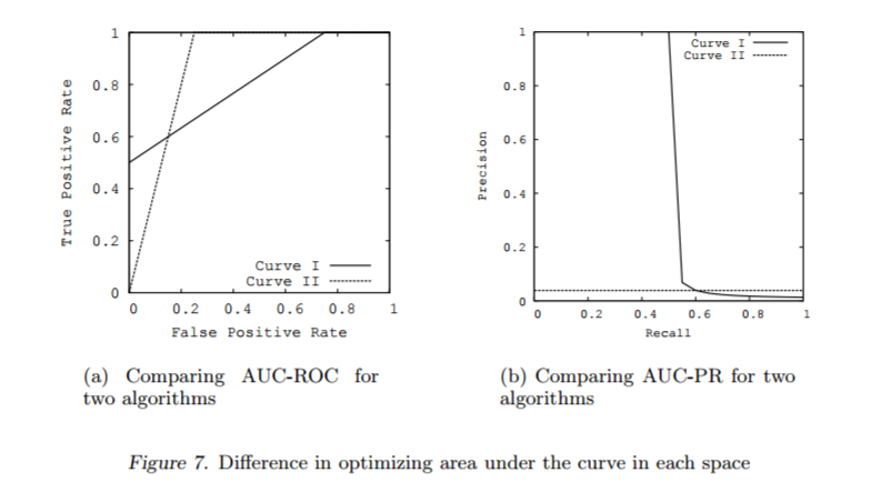
对于不平衡数据集，AUC值是分类器效果评估的常用标准。但如果在解释时不仔细，它也会有一些误导。以Davis and Goadrich (2006)中的模型为例。如图所示，左侧展示的是两个模型的ROC曲线，右侧展示的是precision-recall曲线 (PRC)。

Precision值和Recall值是既矛盾又统一的两个指标，为了提高Precision值，分类器需要尽量在“更有把握”时才把样本预测为正样本，但此时往往会因为过于保守而漏掉很多“没有把握”的正样本，导致Recall值降低。

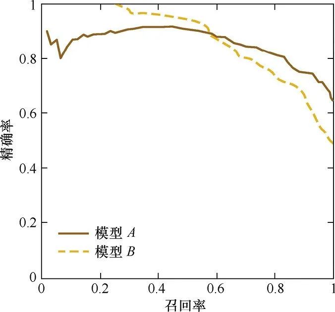
RPC的横轴是召回率，纵轴是精准率。对于一个分类模型来说，其PRC线上的一个点代表着，在某一阈值下，模型将大于该阈值的结果判定为正样本，小于该阈值的结果判定为负样本，此时返回结果对应的召回率和精准率。整条PRC曲线是通过将阈值从高到低移动而生成的。

上图是PRC曲线样例图，其中实线代表模型A的PRC曲线，虚线代表模型B的PRC曲线。原点附近代表当阈值最大时模型的精准率和召回率 (阈值越大，鉴定出的样品越真，能鉴定出的样品越少)。

模型1 (Curve 1)的AUC值为0.813, 模型2 (Curve 2)的AUC值为0.875, 从AUC值角度看模型2更优一点。但是右侧的precision-recall曲线却给出完全不同的结论。模型1 (precision-recall Curve 1)下的面积为0.513，模型2 (precision-recall Curve 2)下的面积为0.038。模型1在较低的假阳性率(FPR<0.2)时有较高的真阳性率。

我们再看另一个关于ROC曲线误导性的例子 Fawcett (2005). 这里有两套数据集：一套为平衡数据集（两类分组为1:1关系），一套为非平衡数据集（两类分组为10:1关系）。每套数据集分别构建2个模型并绘制ROC曲线，从Fig \ref(fig:rocprbalanceimbalance) a,c 可以看出，数据集是否平衡对ROC曲线的影响很小。只是在两个模型之间有一些差别，实线代表的模型在假阳性率较低时 (FPR<0.1)真阳性率低于虚线代表的模型。但precision-recall curve (PRC)曲线却差别很大。对于平衡数据集，两个模型的召回率 (recall)和精准率precision都比较好。对于非平衡数据集，虚线代表的分类模型在较低的召回率时就有较高的精准率。

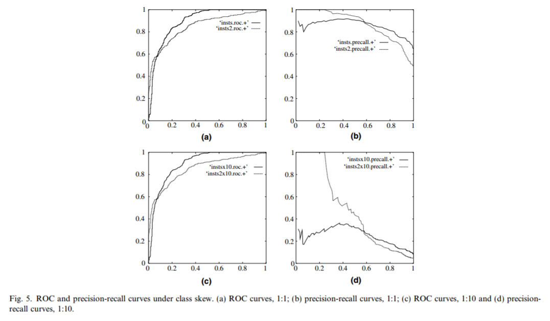
因此，Saito and Rehmsmeier (2015)推荐在处理非平衡数据集时使用PRC曲线，它所反映的信息比ROC曲线更明确。

我们对前面5个模型计算下AUPRC，与AUC结果基本吻合，up效果最好，其次是weighted, smote, down和original。值得差距稍微拉大了一些。

library("PRROC")
calc_auprc <- function(model, data){

  index_class2 <- data$Class == minorityClass
  index_class1 <- data$Class == majorityClass

  predictions <- predict(model, data, type = "prob")

  pr.curve(predictions[[minorityClass]][index_class2],
           predictions[[minorityClass]][index_class1],
           curve = TRUE)

}

# Get results for all 5 models

model_list_pr <- model_list %>%
  map(calc_auprc, data = imbal_test)

model_list_pr %>%
  map(function(the_mod) the_mod$auc.integral)

计算的AUPRC值如下（越大越好）

## $original
## [1] 0.5155589
## 
## $weighted
## [1] 0.640687
## 
## $down
## [1] 0.5302778
## 
## $up
## [1] 0.6461067
## 
## $SMOTE
## [1] 0.6162899

我们绘制PRC曲线观察各个模型的分类效果。基于选定的分类阈值，up sampling和weighting有着最好的精准率和召回率 (单个分组的准确率)。而原始分类器则效果最差。

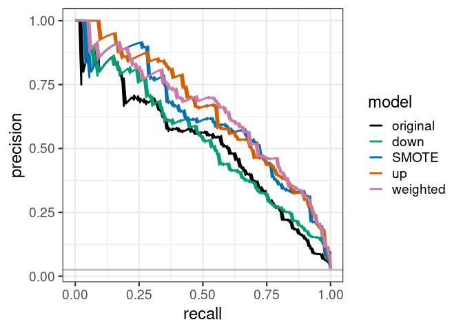
假如加权分类器在召回率 (recall)为75%时，精准率可以达到50% (下面曲线中略低于50%)，则F1得分为0.6。

原始分类器在召回率为75%时，精准率为25% (下面曲线略高于25%)，则F1得分为0.38。

也就是说，当构建好了这两个分类器，并设置一个分类阈值 (不同模型的阈值不同)后，都可以在样品少的分组中获得75%的召回率。但是对于加权模型，有50%的预测为属于样品少的分组的样品是预测对的。而对于原始模型，只有25%预测为属于样品少的分组的样品是预测对的。

# Plot the AUPRC curve for all 5 models

results_list_pr <- list(NA)
num_mod <- 1

for(the_pr in model_list_pr){

  results_list_pr[[num_mod]] <- 
    data_frame(recall = the_pr$curve[, 1],
               precision = the_pr$curve[, 2],
               model = names(model_list_pr)[num_mod])

  num_mod <- num_mod + 1

}

results_df_pr <- bind_rows(results_list_pr)

results_df_pr$model <- factor(results_df_pr$model, 
                               levels=c("original", "down","SMOTE","up","weighted"))

# Plot ROC curve for all 5 models

custom_col <- c("#000000", "#009E73", "#0072B2", "#D55E00", "#CC79A7")

ggplot(aes(x = recall,  y = precision, group = model), data = results_df_pr) +
  geom_line(aes(color = model), size = 1) +
  scale_color_manual(values = custom_col) +
  geom_abline(intercept =
                sum(imbal_test$Class == minorityClass)/nrow(imbal_test),
              slope = 0, color = "gray", size = 1)  +
  theme_bw(base_size = 18) + coord_fixed(1)

基于AUPRC进行调参，修改参数summaryFunction = prSummary和metric = "AUC"。参考https://topepo.github.io/caret/measuring-performance.html （或者看之前的推文）。

# Set up control function for training
ctrlprSummary <- trainControl(method = "repeatedcv",
                     number = 10,
                     repeats = 5,
                     summaryFunction = prSummary,
                     classProbs = TRUE)

# Build a standard classifier using a gradient boosted machine

set.seed(5627)
orig_fit2 <- train(Class ~ .,
                  data = imbal_train,
                  method = "gbm",
                  verbose = FALSE,
                  metric = "AUC",
                  trControl = ctrlprSummary)

# Use the same seed to ensure same cross-validation splits
ctrlprSummary$seeds <- orig_fit$control$seeds

# Build weighted model

weighted_fit2 <- train(Class ~ .,
                      data = imbal_train,
                      method = "gbm",
                      verbose = FALSE,
                      weights = model_weights,
                      metric = "AUC",
                      trControl = ctrlprSummary)

# Build down-sampled model

ctrlprSummary$sampling <- "down"

down_fit2 <- train(Class ~ .,
                  data = imbal_train,
                  method = "gbm",
                  verbose = FALSE,
                  metric = "AUC",
                  trControl = ctrlprSummary)

# Build up-sampled model

ctrlprSummary$sampling <- "up"

up_fit2 <- train(Class ~ .,
                data = imbal_train,
                method = "gbm",
                verbose = FALSE,
                metric = "AUC",
                trControl = ctrlprSummary)

# Build smote model
ctrlprSummary$sampling <- "smote"

smote_fit2 <- train(Class ~ .,
                   data = imbal_train,
                   method = "gbm",
                   verbose = FALSE,
                   metric = "AUC",
                   trControl = ctrlprSummary)

model_list2 <- list(original = orig_fit2,
                   weighted = weighted_fit2,
                   down = down_fit2,
                   up = up_fit2,
                   SMOTE = smote_fit2)

评估下基于prSummary调参后模型的性能，SMOTE处理后的模型效果有提升，其它模型相差不大。

model_list_pr2 <- model_list2 %>%
  map(calc_auprc, data = imbal_test)

model_list_pr2 %>%
  map(function(the_mod) the_mod$auc.integral)

计算的AUPRC值如下（越大越好）

## $original
## [1] 0.5155589
## 
## $weighted
## [1] 0.640687
## 
## $down
## [1] 0.5302778
## 
## $up
## [1] 0.6461067
## 
## $SMOTE
## [1] 0.6341753

绘制PRC曲线

# Plot the AUPRC curve for all 5 models

results_list_pr <- list(NA)
num_mod <- 1

for(the_pr in model_list_pr2){

  results_list_pr[[num_mod]] <- 
    data_frame(recall = the_pr$curve[, 1],
               precision = the_pr$curve[, 2],
               model = names(model_list_pr)[num_mod])

  num_mod <- num_mod + 1

}

results_df_pr <- bind_rows(results_list_pr)

results_df_pr$model <- factor(results_df_pr$model, 
                               levels=c("original", "down","SMOTE","up","weighted"))

# Plot ROC curve for all 5 models

custom_col <- c("#000000", "#009E73", "#0072B2", "#D55E00", "#CC79A7")

ggplot(aes(x = recall,  y = precision, group = model), data = results_df_pr) +
  geom_line(aes(color = model), size = 1) +
  scale_color_manual(values = custom_col) +
  geom_abline(intercept =
                sum(imbal_test$Class == minorityClass)/nrow(imbal_test),
              slope = 0, color = "gray", size = 1)  +
  theme_bw(base_size = 18) + coord_fixed(1)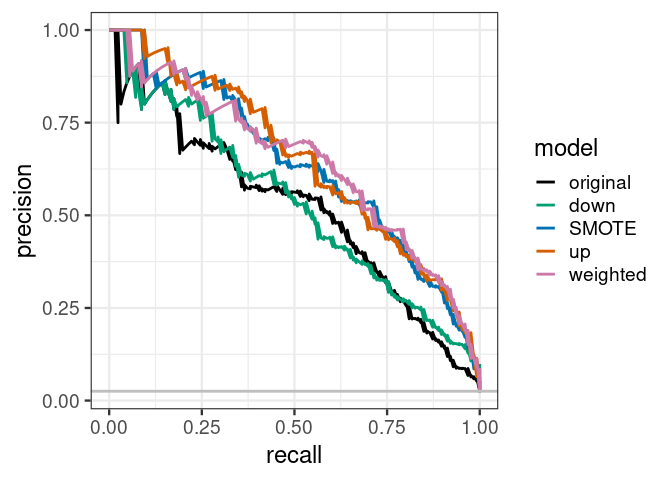

PRC和AUPRC是处理非平衡数据集的有效衡量方式。基于AUC指标来看，权重和重采样技术只带来了微弱的性能提升。但是这个改善更多体现在可以在较低假阳性率基础上获得较高真阳性率，模型的性能更均匀提升。在处理非平衡样本学习问题时，除了尝试调整权重和重采样之外，也不能完全依赖AUC值，而是依靠PRC曲线联合判断，以期获得更好的效果。