异常值检测实践 - Python 代码与可视化

1介绍

.什么是异常值检测？

异常值检测也称为离群值检测、噪声检测、偏差检测或异常挖掘。一般来说并没有普遍接受的定义。（Grubbs，1969）给出的一个早期定义是: 异常值或离群值是似乎与其所在的样本内其他成员明显偏离的观测值。（Barnett 和 Lewis，1994）的最新定义是: 与该组数据的其余部分不一致的观测值。

.成因

导致异常值的最常见原因有，

• 数据输入错误（人为错误）
• 测量误差（仪器误差）
• 实验错误（数据提取或实验计划/执行错误）
• 故意的（虚假的异常值用于测试异常值检测方法）
• 数据处理错误（数据处理或数据集意外突变）
• 抽样错误（从错误或各种不同来源提取或混合数据）
• 自然引入（并不是错误，而是数据多样性导致的数据新颖性）

.应用

异常值/离群值检测的应用比较广泛，例如

• 欺诈检测，即检测信用卡或电话卡的欺诈性事件。
• 贷款申请处理，检测欺诈性申请或潜在问题客户。
• 入侵检测，检测计算机网络中未经授权的访问。
• 活动监视，通过监视电话活动或股票市场中的可疑交易来检测手机欺诈。
• 网络性能，监视计算机网络的性能，例如检测网络瓶颈。
• 故障诊断，检测例如航天飞机上的电动机、发电机、管道或太空仪器中的故障。
• 结构缺陷检测，检测生产线中的缺陷瑕疵。
• 卫星图像分析，识别新颖特征或分类错误的特征。
• 检测图像中的新颖性，用于机器人整形或监视系统。
• 运动分割，检测独立于背景移动的图像特征。
• 时间序列监视，监视安全关键应用，例如钻孔或高速铣削。
• 医疗状况监控，例如心率监控器。
• 药物研究，确定新的分子结构。
• 检测文本中的新颖性，检测新闻事件的出现，进行主题检测和跟踪，或让交易者查明股票、商品、外汇交易事件，表现出色或表现不佳的商品。
• 检测数据库中的意外记录，用于数据挖掘以检测错误、欺诈或有效但异常的记录。
• 在训练数据集中检测标签错误的数据。

.方法

有三类离群值检测方法:

• 在没有数据先验知识的情况下确定异常值。这类似于无监督聚类。
• 对正常和异常进行建模。这类似于监督分类，需要标记好数据。
• 仅建模正常数据。这称为新颖性检测，类似于半监督识别。这种方法需要属于正常类的标记数据。

我将处理第一种方法，这也是最常见的情况。大多数数据集并没有关于异常值的标记数据。

.方法分类

• 离群值检测方法可以分为: 单变量方法和多变量方法。

• 也可以分为: 参数（统计）方法，该类方法假定观测值的潜在分布已知；以及非参数方法，如基于距离的方法和聚类方法。

.离群值检测算法

本篇采用的算法有:

• 孤立森林
• 扩展孤立森林
• 局部离群因子
• DBSCAN
• 单分类 SVM
• 以上方法的集成

2实践

.数据集

这里将使用 Pokemon^[1] 数据集并在 ['HP', 'Speed'] 这两列上执行异常值检测。这个数据集具有很少的观测值，计算将很快。出于可视化目的而只选择了其中两列（二维），但该方法适用于多维度处理。

.上代码

import numpy as np
import pandas as pd
from scipy import stats
import eif as iso
from sklearn import svm
from sklearn.cluster import DBSCAN
from sklearn.ensemble import IsolationForest
from sklearn.neighbors import LocalOutlierFactor

import matplotlib.dates as md
from scipy.stats import norm
%matplotlib inline 
import seaborn as sns 
sns.set_style("whitegrid") #possible choices: white, dark, whitegrid, darkgrid, ticks


import matplotlib.pyplot as plt
plt.style.use('ggplot')
import plotly.express as px
import plotly.graph_objs as go
import plotly.figure_factory as ff
from plotly import tools
from plotly.offline import download_plotlyjs, init_notebook_mode, plot, iplot
pd.set_option('float_format', '{:f}'.format)
pd.set_option('max_columns',250)
pd.set_option('max_rows',150)

data = pd.read_csv('Pokemon.csv')

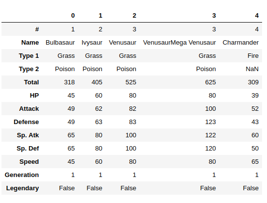
data.head().T

x1='HP'; x2='Speed'
X = data[[x1,x2]]
X.shape

(800, 2)

.孤立森林

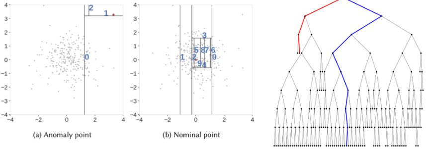
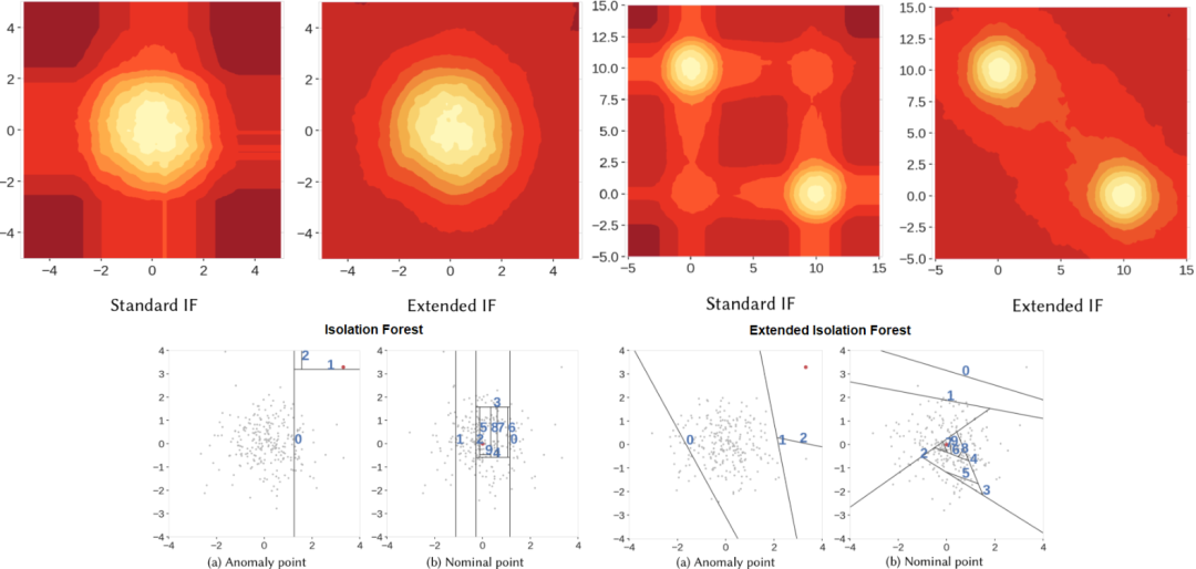
• 孤立森林，就像任何集成树方法一样，都是基于决策树构建的。在这些树中，首先通过随机选择一个特征，然后在所选特征的最小值和最大值之间选择一个随机分割值来创建分区。

• 为了在树中创建分支，首先，选择一个随机特征。然后，为该特征选择一个随机的分割值（介于最小值和最大值之间）。如果给定的观测值具有较低的此特征值，则选择的观测值将归左分支，否则归右分支。继续此过程，直到分割单个点或达到指定的最大深度为止。

• 原则上，离群值不如正常观察值那么普遍，并且在值方面与它们不同（它们离特征空间中的正常观察值更远）。使用这种随机划分，离群值往往出现在更接近树的根的地方，只需相对更少的划分（较短的平均路径长度，即从树的根到叶子节点的边数）。

我将使用 sklearn 库中的 IsolationForest。定义算法时，有一个重要的参数称为污染。它是算法期望的离群值观察值的百分比。我们将 X（具有 HP 和 Speed 2 个特征）拟合到算法中，并在 X 上使用 fit_predict 来对其进行处理。这将产生普通的异常值（-1 为异常值，1 为异常值）。我们还可以使用函数 decision_function 来获得 Isolation Forest 给每个样本的分数。

clf = IsolationForest(max_samples='auto', random_state = 1, contamination= 0.02)

preds = clf.fit_predict(X)

data['isoletionForest_outliers'] = preds
data['isoletionForest_outliers'] = data['isoletionForest_outliers'].astype(str)
data['isoletionForest_scores'] = clf.decision_function(X)

print(data['isoletionForest_outliers'].value_counts())
data[152:156]

1     785
-1     15
Name: isoletionForest_outliers, dtype: int64

将结果绘制出来看看。

fig = px.scatter(data, x=x1, y=x2, color='isoletionForest_outliers', hover_name='Name')
fig.update_layout(title='Isolation Forest Outlier Detection', title_x=0.5, yaxis=dict(gridcolor = '#DFEAF4'), xaxis=dict(gridcolor = '#DFEAF4'), plot_bgcolor='white')
# fig.show()

fig = px.scatter(data, x=x1, y=x2, color="isoletionForest_scores")
fig.update_layout(title='Isolation Forest Outlier Detection (scores)', title_x=0.5,yaxis=dict(gridcolor = '#DFEAF4'), xaxis=dict(gridcolor = '#DFEAF4'), plot_bgcolor='white')
# fig.show()

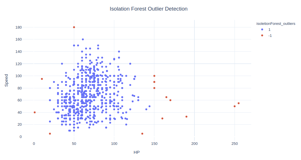
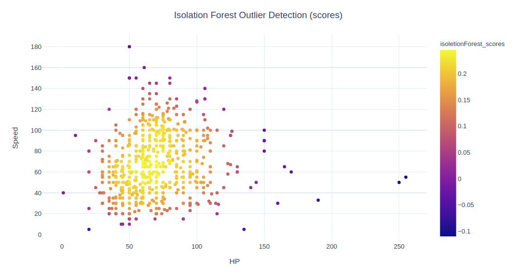
从视觉上看，这 15 个点不在主要数据点范围内，判为离群值似乎合乎常理。

除了异常值和异常值显示孤立森林的决策边界外，我们还可以进行更高级的可视化。

data['isoletionForest_outliers']=='1'

0      True
1      True
2      True
3      True
4      True
       ... 
795    True
796    True
797    True
798    True
799    True
Name: isoletionForest_outliers, Length: 800, dtype: bool

X_inliers = data.loc[data['isoletionForest_outliers']=='1'][[x1,x2]]
X_outliers = data.loc[data['isoletionForest_outliers']=='-1'][[x1,x2]]

xx, yy = np.meshgrid(np.linspace(X.iloc[:, 0].min(), X.iloc[:, 0].max(), 50), np.linspace(X.iloc[:, 1].min(), X.iloc[:, 1].max(), 50))
Z = clf.decision_function(np.c_[xx.ravel(), yy.ravel()])
Z = Z.reshape(xx.shape)

fig, ax = plt.subplots(figsize=(15, 7))
plt.title("Isolation Forest Outlier Detection with Outlier Areas", fontsize = 15, loc='center')
plt.contourf(xx, yy, Z, cmap=plt.cm.Blues_r)

inl = plt.scatter(X_inliers.iloc[:, 0], X_inliers.iloc[:, 1], c='white', s=20, edgecolor='k')
outl = plt.scatter(X_outliers.iloc[:, 0], X_outliers.iloc[:, 1], c='red',s=20, edgecolor='k')

plt.axis('tight')
plt.xlim((X.iloc[:, 0].min(), X.iloc[:, 0].max()))
plt.ylim((X.iloc[:, 1].min(), X.iloc[:, 1].max()))
plt.legend([inl, outl],["normal observations", "abnormal observations"],loc="upper left");
# plt.show()

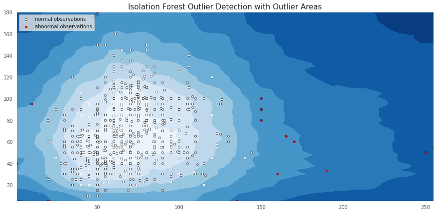
颜色越深，该区域就越离群。下面代码可以查看分数分布。

fig, ax = plt.subplots(figsize=(20, 7))
ax.set_title('Distribution of Isolation Forest Scores', fontsize = 15, loc='center')
sns.distplot(data['isoletionForest_scores'],color='#3366ff',label='if',hist_kws = {"alpha": 0.35});

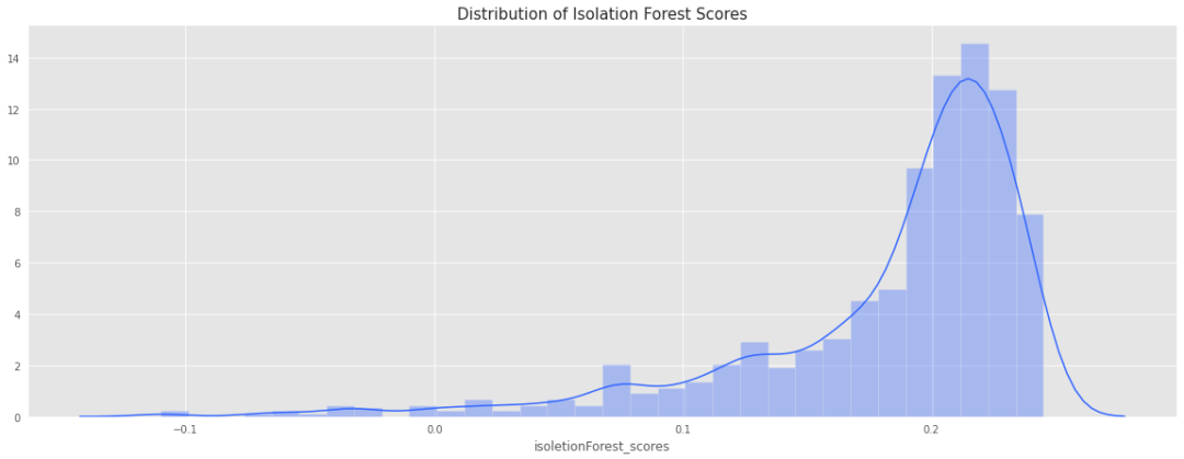
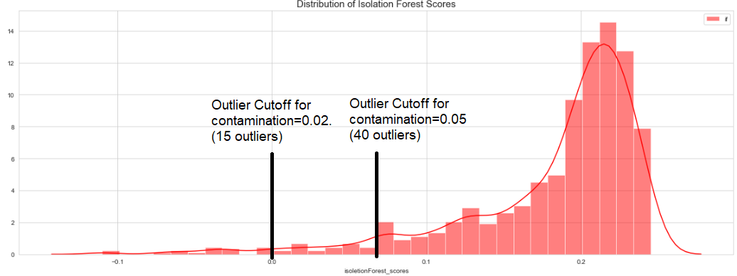
分布很重要，可以帮助我们更好地确定案例的正确污染值。如果我们更改污染值，isoletionForest_scores 将会更改，但是分布将保持不变。该算法将调整分布图中离群值的截止值。

.扩展孤立森林

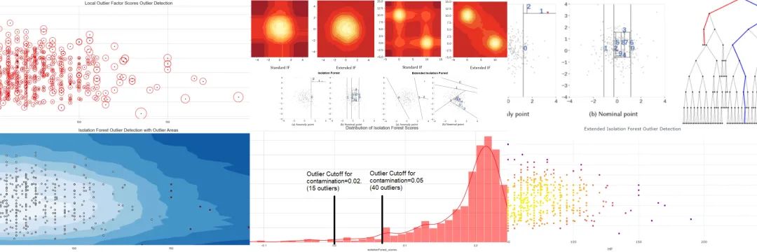
孤立森林有一个缺点: 它的决策边界是垂直或水平的。由于线只能平行于轴，因此某些区域包含许多分支切口，并且只有少量或单个观测值，这会导致某些观测值的异常分不正确。

安装 pip install git+https://github.com/sahandha/eif.git

扩展孤立森林选择如下操作，

X_data = X.values.astype('double')
F1  = iso.iForest(X_data, ntrees=100, sample_size=256, ExtensionLevel=X.shape[1]-1) # X needs to by numpy array
# calculate anomaly scores
anomaly_scores = F1.compute_paths(X_in = X_data)
data['extendedIsoletionForest_scores'] = -anomaly_scores
# determine lowest 2% as outliers
data['extendedIsoletionForest_outliers'] =  data['extendedIsoletionForest_scores'].apply(lambda x: '-1' if x<=data['extendedIsoletionForest_scores'].quantile(0.02) else '1')
print(data['extendedIsoletionForest_outliers'].value_counts())

1     784
-1     16
Name: extendedIsoletionForest_outliers, dtype: int64

fig = px.scatter(data, x=x1, y=x2, color='extendedIsoletionForest_outliers', hover_name='Name')
fig.update_layout(title='Extended Isolation Forest Outlier Detection', title_x=0.5, yaxis=dict(gridcolor = '#DFEAF4'), xaxis=dict(gridcolor = '#DFEAF4'), plot_bgcolor='white')
# fig.show()

fig = px.scatter(data, x=x1, y=x2, color="extendedIsoletionForest_scores")
fig.update_layout(title='Extended Isolation Forest Outlier Detection (scores)', title_x=0.5,yaxis=dict(gridcolor = '#DFEAF4'), xaxis=dict(gridcolor = '#DFEAF4'), plot_bgcolor='white')
# fig.show()

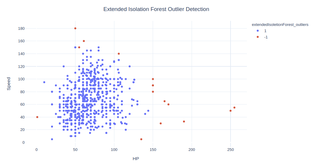
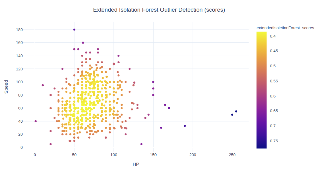
扩展孤立森林并不提供普通的异常值和正常值（如 -1 和 1）。我们只是通过将得分最低的 2％ 作为离群值来创建它们。该算法的分数与基本孤立森林不同，所有分数均为负。

X_inliers = data.loc[data['extendedIsoletionForest_outliers']=='1'][[x1,x2]]
X_outliers = data.loc[data['extendedIsoletionForest_outliers']=='-1'][[x1,x2]]

xx, yy = np.meshgrid(np.linspace(X.iloc[:, 0].min(), X.iloc[:, 0].max(), 50), np.linspace(X.iloc[:, 1].min()-30, X.iloc[:, 1].max()+30, 50))

S1 = F1.compute_paths(X_in=np.c_[xx.ravel(), yy.ravel()])
S1 = S1.reshape(xx.shape)

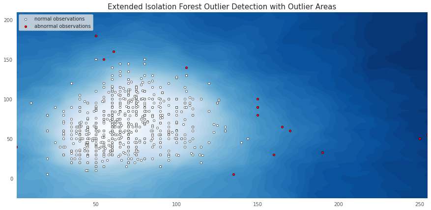
fig, ax = plt.subplots(figsize=(15, 7))
plt.title("Extended Isolation Forest Outlier Detection with Outlier Areas", fontsize = 15, loc='center')
levels = np.linspace(np.min(S1),np.max(S1),50)
CS = ax.contourf(xx, yy, S1, levels, cmap=plt.cm.Blues)

inl = plt.scatter(X_inliers.iloc[:, 0], X_inliers.iloc[:, 1], c='white', s=20, edgecolor='k')
outl = plt.scatter(X_outliers.iloc[:, 0], X_outliers.iloc[:, 1], c='red',s=20, edgecolor='k')

plt.axis('tight')
plt.xlim((X.iloc[:, 0].min(), X.iloc[:, 0].max()))
plt.ylim((X.iloc[:, 1].min()-30, X.iloc[:, 1].max()+30))
plt.legend([inl, outl],["normal observations", "abnormal observations"],loc="upper left")
# plt.show()

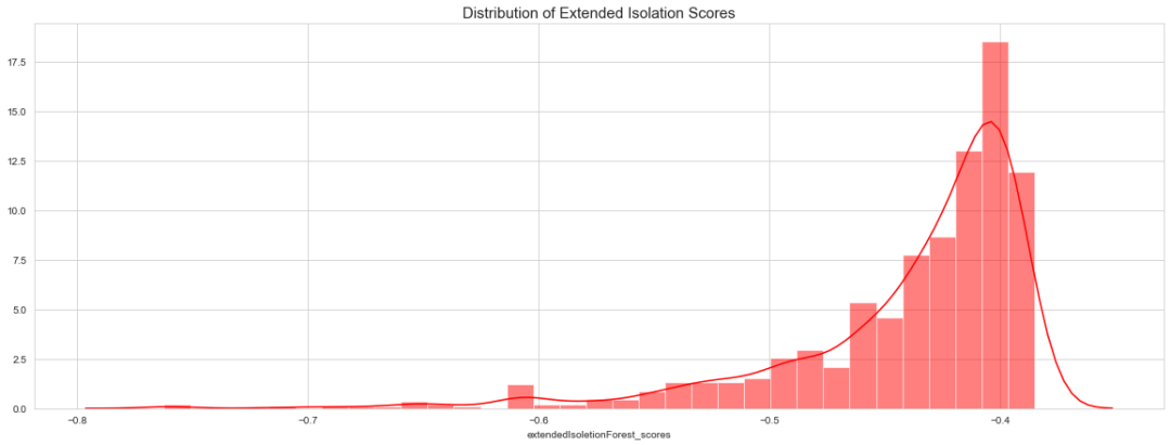
fig, ax = plt.subplots(figsize=(20, 7))
ax.set_title('Distribution of Extended Isolation Scores', fontsize = 15, loc='center')
sns.distplot(data['extendedIsoletionForest_scores'],color='red',label='eif',hist_kws = {"alpha": 0.5});

3局部离群因子 LOF

• 该方法观察某个点的邻近点，找出它的密度，然后将其与其他点的密度进行比较。

• 点的 LOF 表示这个点的密度与其相邻点的密度之比。如果一个点的密度远小于其邻近点的密度（LOF ≫ 1），则该点远离密集区域，判为离群值。

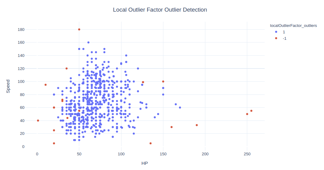
clf = LocalOutlierFactor(n_neighbors=11)
y_pred = clf.fit_predict(X)

data['localOutlierFactor_outliers'] = y_pred.astype(str)
print(data['localOutlierFactor_outliers'].value_counts())
data['localOutlierFactor_scores'] = clf.negative_outlier_factor_

1     779
-1     21
Name: localOutlierFactor_outliers, dtype: int64

最重要的参数是 n_neighbors。默认值为 20，这给出了 45 个离群值。我将其更改为 11 以得到更少的离群值，接近 2％。

fig = px.scatter(data, x=x1, y=x2, color='localOutlierFactor_outliers', hover_name='Name')
fig.update_layout(title='Local Outlier Factor Outlier Detection', title_x=0.5, yaxis=dict(gridcolor = '#DFEAF4'), xaxis=dict(gridcolor = '#DFEAF4'), plot_bgcolor='white')
# fig.show()

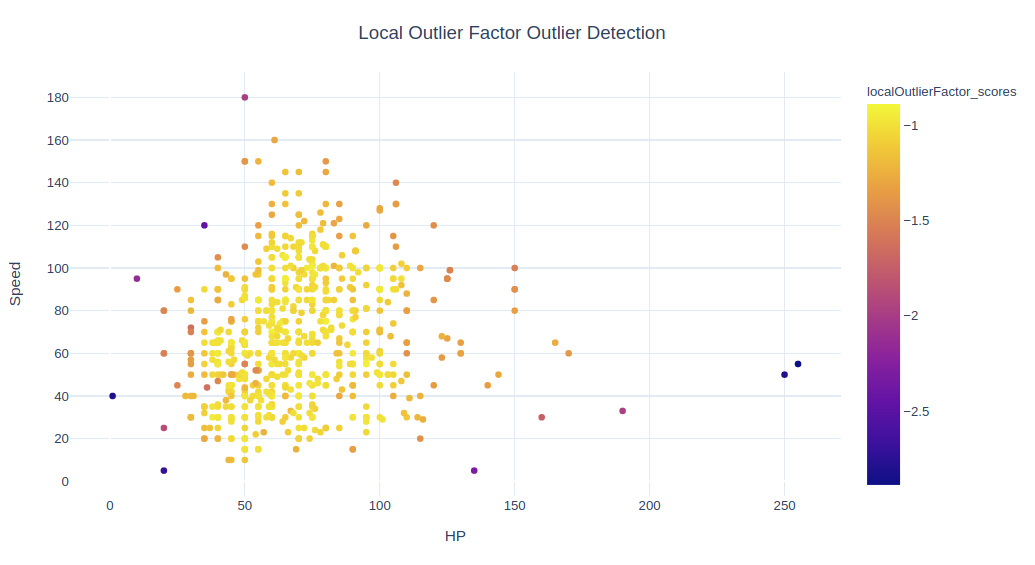
fig = px.scatter(data, x=x1, y=x2, color="localOutlierFactor_scores", hover_name='Name')
fig.update_layout(title='Local Outlier Factor Outlier Detection', title_x=0.5,yaxis=dict(gridcolor = '#DFEAF4'), xaxis=dict(gridcolor = '#DFEAF4'), plot_bgcolor='white')
# fig.show()

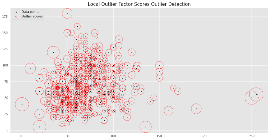
我们可以创建另一个有趣的图，其中局部离群值越大，其周围的圆圈越大。

fig, ax = plt.subplots(figsize=(15, 7.5))
ax.set_title('Local Outlier Factor Scores Outlier Detection', fontsize = 15, loc='center')

plt.scatter(X.iloc[:, 0], X.iloc[:, 1], color='k', s=3., label='Data points')
radius = (data['localOutlierFactor_scores'].max() - data['localOutlierFactor_scores']) / (data['localOutlierFactor_scores'].max() - data['localOutlierFactor_scores'].min())
plt.scatter(X.iloc[:, 0], X.iloc[:, 1], s=2000 * radius, edgecolors='r', facecolors='none', label='Outlier scores')
plt.axis('tight')
legend = plt.legend(loc='upper left')
legend.legendHandles[0]._sizes = [10]
legend.legendHandles[1]._sizes = [20]
plt.show();

fig, ax = plt.subplots(figsize=(20, 7))
ax.set_title('Distribution of Local Outlier Factor Scores', fontsize = 15, loc='center')
sns.distplot(data['localOutlierFactor_scores'],color='red',label='eif',hist_kws = {"alpha": 0.5});

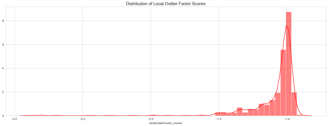
该算法与以前的算法有很大不同，它以不同的方式找到离群值。

.DBSCAN

一种经典的聚类算法，其工作方式如下：

• 随机选择一个尚未分配给簇或指定为离群值的点。通过查看 epsilon 距离内是否至少有 min_samples 个点来确定其是否为核心点。

• 将核心点及其在 epsilon 距离内的所有直接可达点构成一簇。

• 查找簇中每个点的 epsilon 距离内的所有点，并将它们添加到该簇中。查找所有新添加的点在 epsilon 距离内的所有点，并将它们添加到簇中。重复上述步骤。

from sklearn.cluster import DBSCAN
outlier_detection = DBSCAN(eps = 20, metric='euclidean', min_samples = 5,n_jobs = -1)
clusters = outlier_detection.fit_predict(X)

data['dbscan_outliers'] = clusters
data['dbscan_outliers'] = data['dbscan_outliers'].apply(lambda x: str(1) if x>-1 else str(-1))
print(data['dbscan_outliers'].value_counts())

1     787
-1     13
Name: dbscan_outliers, dtype: int64

要调整的最重要参数是 eps。

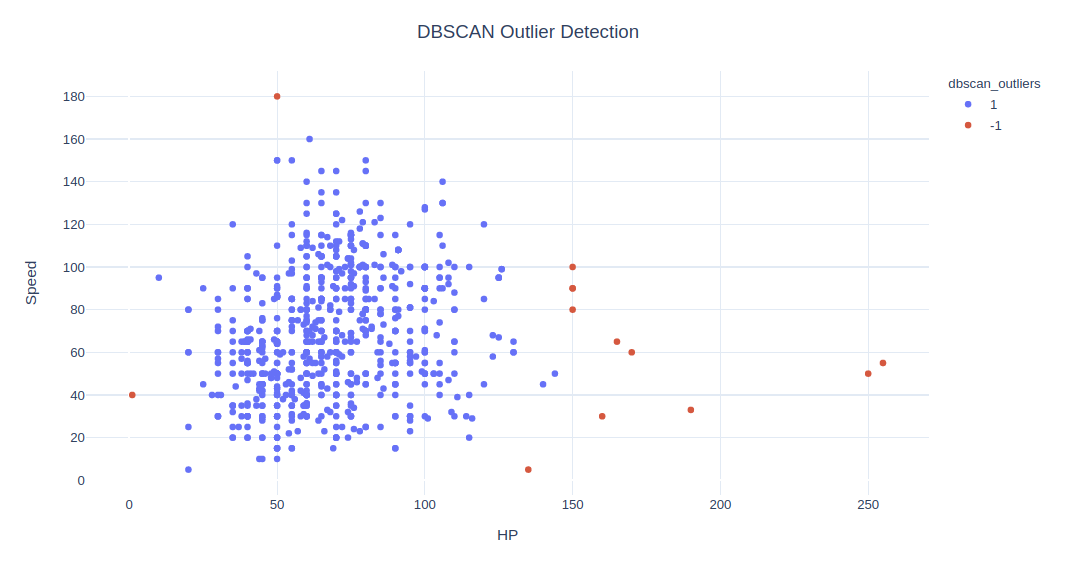
fig = px.scatter(data, x=x1, y=x2, color="dbscan_outliers", hover_name='Name')
fig.update_layout(title='DBSCAN Outlier Detection', title_x=0.5,yaxis=dict(gridcolor = '#DFEAF4'), xaxis=dict(gridcolor = '#DFEAF4'), plot_bgcolor='white')
# fig.show()

.单分类 SVM

• 单类分类器在仅包含正常点的数据集上训练，但可用于所有数据。一旦训练好，该模型将用于将新示例分类为正常值或异常值。

• 与标准 SVM 的主要区别在于，它以无监督的方式拟合，并不提供超参数 C 来调节间隔。相反，它提供了控制支持向量灵敏度的超参数 nu，并且应该调整为数据中离群值的近似比率。

有关单分类 SVM 的更多信息可参考，

• Outlier Detection with One-Class SVMs^[2]
• One-Class Classification Algorithms for Imbalanced Datasets^[3]

clf = svm.OneClassSVM(nu=0.08, kernel='rbf', gamma='auto')
outliers = clf.fit_predict(X)
data['ocsvm_outliers'] = outliers
data['ocsvm_outliers'] = data['ocsvm_outliers'].apply(lambda x: str(-1) if x==-1 else str(1))
data['ocsvm_scores'] = clf.score_samples(X)
print(data['ocsvm_outliers'].value_counts())

-1    481
1     319
Name: ocsvm_outliers, dtype: int64

fig = px.scatter(data, x=x1, y=x2, color="ocsvm_outliers", hover_name='Name')
fig.update_layout(title='One Class SVM Outlier Detection', title_x=0.5,yaxis=dict(gridcolor = '#DFEAF4'), xaxis=dict(gridcolor = '#DFEAF4'), plot_bgcolor='white')
# fig.show()

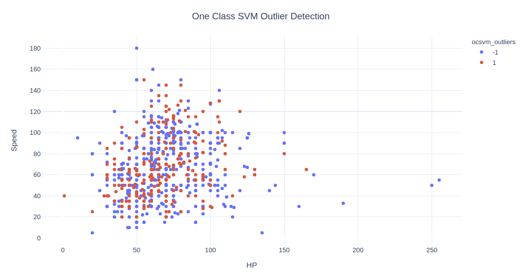
在此数据中找不到更好的 nu，参数在这个例子上似乎不起作用。对于其他 nu 值，离群值更是大于正常值。

.集成

最后，让我们结合这 5 种算法来构成一种健壮的算法。我将简单添加离群值列，其中 -1 代表离群值，1 代表正常值。

由于此例中效果不好，因此不使用 One Class SVM。

data['outliers_sum'] = data['isoletionForest_outliers'].astype(int)+data['extendedIsoletionForest_outliers'].astype(int)+data['localOutlierFactor_outliers'].astype(int)+data['dbscan_outliers'].astype(int)

data['outliers_sum'].value_counts()

 3    774
 1     11
-3      8
-1      7
Name: outliers_sum, dtype: int64

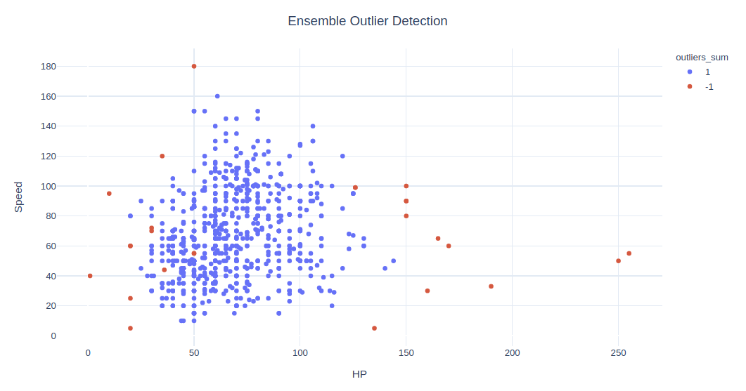
fig = px.scatter(data, x=x1, y=x2, color="outliers_sum", hover_name='Name')
fig.update_layout(title='Ensemble Outlier Detection', title_x=0.5,yaxis=dict(gridcolor = '#DFEAF4'), xaxis=dict(gridcolor = '#DFEAF4'), plot_bgcolor='white')
# fig.show()

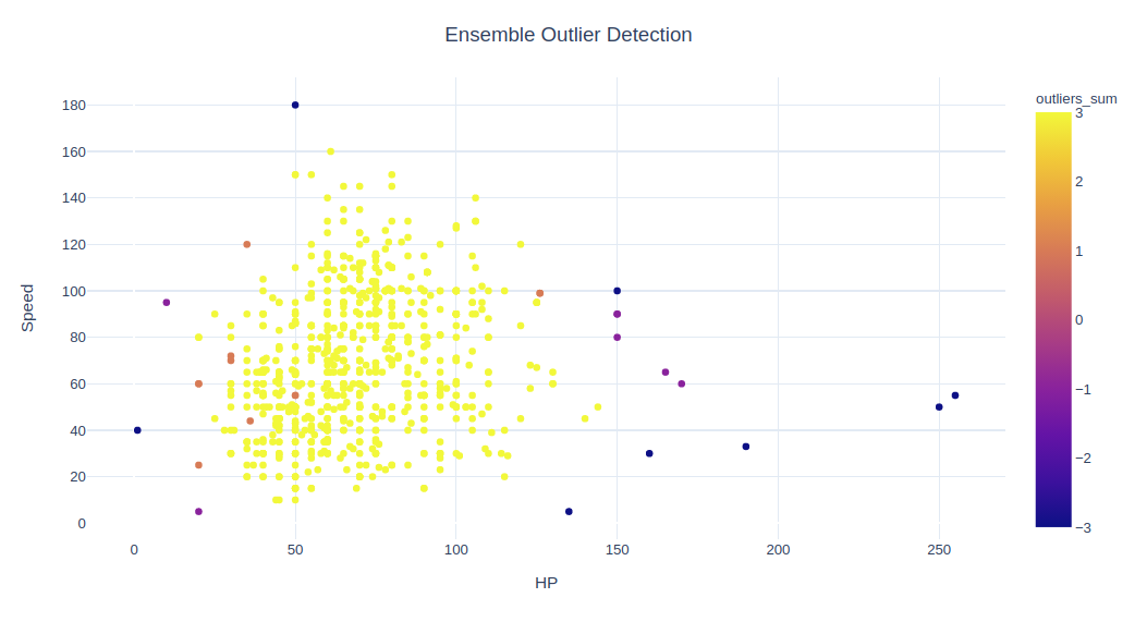
观察值 outliers_sum=4 的意思是，所有 4 种算法均同意这是一个正常值，而对于离群值的完全一致是其和为 -4。

首先，让我们看看所有算法中哪些被认为是离群值，然后将 sum = 4 的观察值设为正常值，其余则作为离群值。

data.loc[data['outliers_sum']==-4]['Name']

121              Chansey
155              Snorlax
217            Wobbuffet
261              Blissey
313              Slaking
316             Shedinja
431    DeoxysSpeed Forme
495             Munchlax
Name: Name, dtype: object

data['outliers_sum'] = data['outliers_sum'].apply(lambda x: str(1) if x==4 else str(-1))

fig = px.scatter(data, x=x1, y=x2, color="outliers_sum", hover_name='Name')
fig.update_layout(title='Ensemble Outlier Detection', title_x=0.5,yaxis=dict(gridcolor = '#DFEAF4'), xaxis=dict(gridcolor = '#DFEAF4'), plot_bgcolor='white')
# fig.show()

⟳参考资料⟲

.相关阅读