21 句话入门机器学习！-技术圈

来源：CSDN博客算法进阶

对于程序员来说，机器学习的重要性毋庸赘言。也许你还没有开始，也许曾经失败过，都没有关系，你将在这里找到或者重拾自信。只要粗通Python，略知NumPy，认真读完这21句话，逐行敲完示例代码，就可以由此进入自由的AI王国。

机器学习有四种用途：分类、聚类、回归和降维。更严格一点，机器学习的目的只有三个：分类、聚类和回归，降维不过是达成目标的手段之一。

分类和聚类都是对个体样本归类，看起来很相似，实则相去甚远——前者属于有监督的学习，后者属于无监督的学习。

分类是基于经验的，而经验来自过往的数据，这意味着分类需要训练；聚类则是基于当前全部样本的特征，不依赖经验，自然也就无需训练。举个例子：让你从一堆水果中挑出苹果、橘子和香蕉，这是分类；让你将画在纸上的若干个图案分组，分组规则由你决定，这是聚类。

从字面上看，分类和回归看上去风马牛不相及，其实二者是亲兄弟，使用的算法几乎完全重合。

分类是对个体样本做出定性判定，回归是对个体样本做出定量判定，二者同属于有监督的学习，都是基于经验的。举个例子：有经验的老师预测某学生考试及格或不及格，这是分类；预测某学生能考多少分，这是回归；不管是预测是否及格还是预测考多少分，老师的经验数据和思考方法是相同的，只是最后的表述不同而已。

传统的软件开发，代码是重点，而对于机器学习，数据是重点。

在训练机器学习模型时，数据的质量和数量都会影响训练结果的准确性和有效性。因此，无论是学习还是应用机器学习模型解决问题，前提都是要有足够多且足够好的数据集。

数据集通常是指由若干个样本数据组成的二维数组，数组的每一行表示一个样本的数据。

举个例子：用性别、年龄、身高（米）、体重（千克）、职业、年薪（万元）、不动产（万元）、有价证券（万元）等信息组成的一维数组表示一位征婚者的数据，下面的二维数组就是一个婚介机构收集到的征婚者数据集。

>>> import numpy as np>>> members = np.array([  ['男', '25', 185, 80, '程序员', 35, 200,  30],  ['女', '23', 170, 55, '公务员', 15,   0,  80],  ['男', '30', 180, 82, '律师',   60, 260, 300],  ['女', '27', 168, 52, '记者',   20, 180, 150]])

数据集的列，也被成为特征维或特征列。

上面的征婚者数据集共有性别、年龄、身高（米）、体重（千克）、职业、年薪（万元）、不动产（万元）、有价证券（万元）等8列，也可以说这个数据集有8个特征维或特征列。

所谓降维，并非是将数据集从二维变成一维，而是减少数据集的特征维。

征婚者的个人信息远不止上面所列出的这8项，还可以加上生日、业余爱好、喜欢的颜色、爱吃的食物等等。不过，要是将所有的个人信息都加入到数据集中，不但会增加数据保存和处理的难度和成本，对于择偶者来说，也会因为信息量太多而分散了注意力，以至于忽略了最重要的信息。降维就是从数据集中剔除对结果无影响或影响甚微的特征列。

标准化是对样本集的每个特征列减去该特征列的平均值进行中心化，再除以标准差进行缩放。

满分为100分的考试中，你如果得了90分，这自然是一个好成绩。不过要是和其他同学比的话，就未必是了：假如其他同学都是满分，那90分就是最差的一个。数据标准化的意义在于反映个体数据偏离所有样本平均值的程度。下面是对征婚者数据集中有价证券特征列标准化后的结果。

>>> security = np.float32((members[:,-1])) # 提取有价证券特征列数据>>> securityarray([ 30.,  80., 300., 150.], dtype=float32)>>> (security - security.mean())/security.std() # 减去均值再除以标准差array([-1.081241, -0.5897678, 1.5727142, 0.09829464], dtype=float32)

归一化是对样本集的每个特征列减去该特征列的最小值进行中心化，再除以极差（最大值最小值之差）进行缩放。

归一化处理类似于标准化，结果收敛于[0,1]区间内。下面是对征婚者数据集中有价证券特征列归一化后的结果。

>>> security = np.float32((members[:,-1])) # 提取有价证券特征列数据>>> securityarray([ 30.,  80., 300., 150.], dtype=float32)>>> (security - security.min())/(security.max() - security.min()) # 减去最小值再除以极差array([0., 0.18518518, 1., 0.44444445], dtype=float32)

机器学习模型只能处理数值数据，因此需要将性别、职业等非数值数据变成整数，这个过程被称为特征编码。

征婚者数据集中，对于性别特征列，可以用0表示女性，用1表示男性，或者反过来也没有问题。不过这个方法不适用于职业特征列的编码，因为不同职业之间原本是无序的，如果用这个方法编码，就会产生2比1更接近3的问题。此时通行的做法是使用独热码（one-of-K）：若有n个不同的职业，就用n位二进制数字表示，每个数字只有1位为1其余为0。此时，职业特征列将从1个扩展为n个。下面使用Scikit-learn的独热码编码器对性别和职业两列做特征编码，生成6个特征列（性别2列，职业4列）。该编码器位于preprocessing子模块中。

>>> from sklearn import preprocessing as pp>>> X = [  ['男', '程序员'],  ['女', '公务员'],  ['男', '律师', ],  ['女', '记者', ]]>>> ohe = pp.OneHotEncoder().fit(X)>>> ohe.transform(X).toarray()array([[0., 1., 0., 0., 1., 0.],       [1., 0., 1., 0., 0., 0.],       [0., 1., 0., 1., 0., 0.],       [1., 0., 0., 0., 0., 1.]])

Scikit-learn的数据集子模块datasets提供了若干数据集：函数名以load 开头的是模块内置的小型数据集；函数名以fetch开头，是需要从外部数据源下载的大型数据集。

datasets.load_boston([return_X_y]) ：加载波士顿房价数据集datasets.load_breast_cancer([return_X_y]) ：加载威斯康星州乳腺癌数据集datasets.load_diabetes([return_X_y]) ：加载糖尿病数据集datasets.load_digits([n_class, return_X_y]) ：加载数字数据集datasets.load_iris([return_X_y]) ：加载鸢尾花数据集。datasets.load_linnerud([return_X_y]) ：加载体能训练数据集datasets.load_wine([return_X_y]) ：加载葡萄酒数据集datasets.fetch_20newsgroups([data_home, …]) ：加载新闻文本分类数据集datasets.fetch_20newsgroups_vectorized([…]) ：加载新闻文本向量化数据集datasets.fetch_california_housing([…]) ：加载加利福尼亚住房数据集datasets.fetch_covtype([data_home, …]) ：加载森林植被数据集datasets.fetch_kddcup99([subset, data_home, …]) ：加载网络入侵检测数据集datasets.fetch_lfw_pairs([subset, …]) ：加载人脸（成对）数据集datasets.fetch_lfw_people([data_home, …]) ：加载人脸（带标签）数据集datasets.fetch_olivetti_faces([data_home, …]) ：加载 Olivetti 人脸数据集datasets.fetch_rcv1([data_home, subset, …])：加载路透社英文新闻文本分类数据集datasets.fetch_species_distributions([…]) ：加载物种分布数据集

每个二维的数据集对应着一个一维的标签集，用于标识每个样本的所属类别或属性值。通常数据集用大写字母X表示，标签集用小写字母y表示。

下面的代码从数据集子模块datasets中提取了鸢尾花数据集——这是用来演示分类模型的最常用的数据集。鸢尾花数据集X共有150个样本，每个样本有4个特征列，分别使花萼的长度和宽度、花瓣的长度和宽度。这些样本共有3种类型，分别用整数0、1、2表示，所有样本的类型标签组成标签集y，这是一个一维数组。

>>> from sklearn.datasets import load_iris>>> X, y = load_iris(return_X_y=True)>>> X.shape # 数据集X有150个样本，4个特征列(150, 4)>>> y.shape # 标签集y的每一个标签和数据集X的每一个样本一一对应(150,)>>> X[0], y[0](array([5.1, 3.5, 1.4, 0.2]), 0)

加载数据时，如果指定return_X_y参数为False（默认值），则可以查看标签的名字。

>>> iris = load_iris()>>> iris.target_names # 查看标签的名字array(['setosa', 'versicolor', 'virginica'], dtype='<U10')>>> X = iris.data>>> y = iris.target

模型训练时，通常会将数据集和标签集分成两部分：一部分用于训练，一部分用于测试。

分割数据集是一项非常重要的工作，不同的分割方法对于模型训练的结果有不同的影响。Scikit-learn提供了很多种数据集分割方法，train_test_split是其中最简单的一种，可以根据指定的比例随机抽取测试集。train_test_split函数位于模型选择子模块model_selection中。

>>> from sklearn.datasets import load_iris>>> from sklearn.model_selection import train_test_split as tsplit>>> X, y = load_iris(return_X_y=True)>>> X_train, X_test, y_train, y_test = tsplit(X, y, test_size=0.1)>>> X_train.shape, X_test.shape((135, 4), (15, 4))>>> y_train.shape, y_test.shape((135,), (15,))

上面的代码按照10%的比例随机从数据集中抽取样本作为测试集，剩余样本作为训练集。分割完成后，训练集有135个样本，测试集有15个样本。

近朱者赤，近墨者黑，距离谁最近，就和谁同类——这就是k-近邻分类。

k-近邻分类是最简单、最容易的分类方法。对于待分类的样本，从训练集中找出k个和它距离最近的样本，考察这些样本中哪一个标签最多，就给待分类样本贴上该标签。k值的最佳选择高度依赖数据，较大的k值会抑制噪声的影响，但同时也会使分类界限不明显。通常k值选择不大于20的整数。

>>> from sklearn.datasets import load_iris>>> from sklearn.model_selection import train_test_split as tsplit>>> from sklearn.neighbors import KNeighborsClassifier # 导入k-近邻分类模型>>> X, y = load_iris(return_X_y=True) # 获取鸢尾花数据集，返回样本集和标签集>>> X_train, X_test, y_train, y_test = tsplit(X, y, test_size=0.1) # 拆分为训练集和测试集>>> m = KNeighborsClassifier(n_neighbors=10) # 模型实例化，n_neighbors参数指定k值，默认k=5>>> m.fit(X_train, y_train) # 模型训练KNeighborsClassifier()>>> m.predict(X_test) # 对测试集分类array([2, 1, 2, 2, 1, 2, 1, 2, 2, 1, 0, 1, 0, 0, 2])>>> y_test # 这是实际的分类情况，上面的预测只错了一个array([2, 1, 2, 2, 2, 2, 1, 2, 2, 1, 0, 1, 0, 0, 2])>>> m.score(X_test, y_test) # 模型测试精度（介于0~1）0.9333333333333333

应用分类模型对15个测试样本分类，结果只有1个是错误的，准确率约为93%。在分类算法中，score是最常用的评估函数，返回分类正确的样本数与测试样本总数之比。

一辆开了八年的大切诺基可以卖多少钱？最简单的方法是参考k辆同款车型且使用年限相近的二手车售价的均值——这就是k-近邻回归。

k-近邻算法不仅可以用来解决分类问题，也可以用来解决回归问题。k-近邻回归预测样本的标签由它最近邻标签的均值计算而来。下面的代码以波士顿房价数据集为例，演示了k-近邻回归模型的用法。波士顿房价数据集统计的是20世纪70年代中期波士顿郊区房价的中位数，一共有506条不同的数据，每条数据包含区域的人文环境、自然环境、商业环境、交通状况等13个属性，标签是区域房价的平均值。

>>> from sklearn.datasets import load_boston>>> from sklearn.model_selection import train_test_split as tsplit>>> from sklearn.neighbors import KNeighborsRegressor>>> X, y = load_boston(return_X_y=True) # 加载波士顿房价数据集>>> X.shape, y.shape, y.dtype # 该数据集共有506个样本，13个特征列，标签集为浮点型，适用于回归模型((506, 13), (506,), dtype('float64'))>>> X_train, X_test, y_train, y_test = tsplit(X, y, test_size=0.01) # 拆分为训练集和测试集>>> m = KNeighborsRegressor(n_neighbors=10) # 模型实例化，n_neighbors参数指定k值，默认k=5>>> m.fit(X_train, y_train) # 模型训练KNeighborsRegressor(n_neighbors=10)>>> m.predict(X_test) # 预测6个测试样本的房价array([27.15, 31.97, 12.68, 28.52, 20.59, 21.47])>>> y_test # 这是测试样本的实际价格，除了第2个（索引为1）样本偏差较大，其他样本偏差还算差强人意array([29.1, 50. , 12.7, 22.8, 20.4, 21.5])

常用的回归模型的评价方法有均方误差、中位数绝对误差和复相关系数等。

评价一个回归结果的优劣，比评价一个分类结果要困难得多——前者需要考虑偏离程度，而后者只考虑对错。常用的回归评价函数是均方误差函数、中位数绝对误差函数和复相关系数函数等，这几个函数均被包含在模型评估指标子模块metrics中。均方误差和中位数绝对误差越小，说明模型精确度越高；复相关系数则相反，越接近1说明模型精确度越高，越接近0说明模型越不可用。

以上一段代码为例，模型评估结果如下。

>>> from sklearn import metrics>>> y_pred = m.predict(X_test)>>> metrics.mean_squared_error(y_test, y_pred) # 均方误差60.27319999999995>>> metrics.median_absolute_error(y_test, y_pred) # 中位数绝对误差1.0700000000000003>>> metrics.r2_score(y_test, y_pred) # 复相关系数0.5612816401629652

复相关系数只有0.56，显然，用k-近邻算法预测波士顿房价不是一个好的选择。下面的代码尝试用决策树算法预测波士顿房价，得到了较好的效果，复相关系数达到0.98，预测房价非常接近实际价格，误差极小。

>>> from sklearn.datasets import load_boston>>> from sklearn.model_selection import train_test_split as tsplit>>> from sklearn.tree import DecisionTreeRegressor>>> X, y = load_boston(return_X_y=True) # 加载波士顿房价数据集>>> X_train, X_test, y_train, y_test = tsplit(X, y, test_size=0.01) # 拆分为训练集和测试集>>> m = DecisionTreeRegressor(max_depth=10) # 实例化模型，决策树深度为10>>> m.fit(X, y) # 训练DecisionTreeRegressor(max_depth=10)>>> y_pred = m.predict(X_test) # 预测>>> y_test # 这是测试样本的实际价格，除了第2个（索引为1）样本偏差略大，其他样本偏差较小array([20.4,  21.9,  13.8,  22.4, 13.1,  7. ])>>> y_pred # 这是6个测试样本的预测房价，非常接近实际价格array([20.14, 22.33, 14.34, 22.4, 14.62, 7. ])>>> metrics.r2_score(y_test, y_pred) # 复相关系数0.9848774474870712>>> metrics.mean_squared_error(y_test, y_pred) # 均方误差0.4744784865112032>>> metrics.median_absolute_error(y_test, y_pred) # 中位数绝对误差0.3462962962962983

决策树、支持向量机（SVM）、贝叶斯等算法，既可以解决分类问题，也可以解决回归问题。

应用这些算法解决分类和回归问题的流程，与使用k-近邻算法基本相同，不同之处在于不同的算法提供了不同的参数。我们需要仔细阅读算法文档，搞清楚这些参数的含义，选择正确的参数，才有可能得到正确的结果。比如，支持向量机（SVM）的回归模型参数中，比较重要的有kernel参数和C参数。kernel参数用来选择内核算法；C是误差项的惩罚参数，取值一般为10的整数次幂，如 0.001、0.1、1000 等。通常，C值越大，对误差项的惩罚越大，因此训练集测试时准确率就越高，但泛化能力越弱；C值越小，对误差项的惩罚越小，因此容错能力越强，泛化能力也相对越强。

下面的例子以糖尿病数据集为例，演示了支持向量机（SVM）回归模型中不同的C参数对回归结果的影响。糖尿病数据集收集了442 例糖尿病患者的10 个指标（年龄、性别、体重指数、平均血压和6 个血清测量值），标签是一年后疾病进展的定量测值。需要特别指出，糖尿病数据集并不适用于SVM算法，此处仅是为了演示参数选择如何影响训练结果。

>>> from sklearn.datasets import load_diabetes>>> from sklearn.model_selection import train_test_split as tsplit>>> from sklearn.svm import SVR>>> from sklearn import metrics>>> X, y = load_diabetes(return_X_y=True)>>> X.shape, y.shape, y.dtype((442, 10), (442,), dtype('float64'))>>> X_train, X_test, y_train, y_test = tsplit(X, y, test_size=0.02)>>> svr_1 = SVR(kernel='rbf', C=0.1) # 实例化SVR模型，rbf核函数，C=0.1>>> svr_2 = SVR(kernel='rbf', C=100) # 实例化SVR模型，rbf核函数，C=100>>> svr_1.fit(X_train, y_train) # 模型训练SVR(C=0.1)>>> svr_2.fit(X_train, y_train) # 模型训练SVR(C=100)>>> z_1 = svr_1.predict(X_test) # 模型预测>>> z_2 = svr_2.predict(X_test) # 模型预测>>> y_test # 这是测试集的实际值array([ 49., 317.,  84., 181., 281., 198.,  84.,  52., 129.])>>> z_1 # 这是C=0.1的预测值，偏差很大array([138.10720127, 142.1545034 , 141.25165838, 142.28652449,       143.19648143, 143.24670732, 137.57932272, 140.51891989,       143.24486911])>>> z_2 # 这是C=100的预测值，偏差明显变小array([ 54.38891948, 264.1433666 , 169.71195204, 177.28782561,       283.65199575, 196.53405477,  61.31486045, 199.30275061,       184.94923477])>>> metrics.mean_squared_error(y_test, z_1) # C=0.01的均方误差8464.946517460194>>> metrics.mean_squared_error(y_test, z_2) # C=100的均方误差3948.37754995066>>> metrics.r2_score(y_test, z_1) # C=0.01的复相关系数0.013199351909129464>>> metrics.r2_score(y_test, z_2) # C=100的复相关系数0.5397181166871942>>> metrics.median_absolute_error(y_test, z_1) # C=0.01的中位数绝对误差57.25165837797314>>> metrics.median_absolute_error(y_test, z_2) # C=100的中位数绝对误差22.68513954888364

随机森林是将多棵分类决策树或者回归决策树集成在一起的算法，是机器学习的一个分支——集成学习的方法。

以随机森林分类为例，随机森林包含的每棵决策树都是一个分类模型，对于一个输入样本，每个分类模型都会产生一个分类结果，类似投票表决。随机森林集成了所有的投票分类结果，并将被投票次数最多的类别指定为最终的输出类别。随机森林每颗决策树的训练样本都是随机的，决策树中训练集的特征列也是随机选择确定的。正是因为这两个随机性的存在，使得随机森林不容易陷入过拟合，并且具有很好的抗噪能力。

考虑到随机森林的每一棵决策树中训练集的特征列是随机选择确定的，更适合处理具有多特征列的数据，这里选择 Scikit-learn内置的威斯康星州乳腺癌数据集来演示随机森林分类模型的使用。该数据集有 569 个乳腺癌样本，每个样本包含半径、纹理、周长、面积、是否平滑、是否紧凑、是否凹凸等 30 个特征列。

>>> from sklearn.datasets import load_breast_cancer # 导入数据加载函数>>> from sklearn.tree import DecisionTreeClassifier # 导入随机树>>> from sklearn.ensemble import RandomForestClassifier # 导入随机森林>>> from sklearn.model_selection import cross_val_score # 导入交叉验证>>> ds = load_breast_cancer() # 加载威斯康星州乳腺癌数据集>>> ds.data.shape # 569个乳腺癌样本，每个样本包含30个特征(569, 30)>>> dtc = DecisionTreeClassifier() # 实例化决策树分类模型>>> rfc = RandomForestClassifier() # 实例化随机森林分类模型>>> dtc_scroe = cross_val_score(dtc, ds.data, ds.target, cv=10) # 交叉验证>>> dtc_scroe # 决策树分类模型交叉验证10次的结果array([0.92982456, 0.85964912, 0.92982456, 0.89473684, 0.92982456,       0.89473684, 0.87719298, 0.94736842, 0.92982456, 0.92857143])>>> dtc_scroe.mean() # 决策树分类模型交叉验证10次的平均精度0.9121553884711779>>> rfc_scroe = cross_val_score(rfc, ds.data, ds.target, cv=10) # 交叉验证>>> rfc_scroe # 随机森林分类模型交叉验证10次的结果array([0.98245614, 0.89473684, 0.94736842, 0.94736842, 0.98245614,       0.98245614, 0.94736842, 0.98245614, 0.94736842, 1.        ])>>> rfc_scroe.mean()# 随机森林分类模型交叉验证10次的平均精度0.9614035087719298

上面的代码使用了交叉验证法，其原理是将样本分成n份，每次用其中的n-1份作训练集，剩余1份作测试集，训练n次，返回每次的训练结果。结果显示，同样交叉验证10次，96%对91%，随机森林的分类准确率明显高于随机树。

基于质心的聚类，无论是k均值聚类还是均值漂移聚类，其局限性都是显而易见的：无法处理细长条、环形或者交叉的不规则的样本分布。

k均值（k-means）聚类通常被视为聚类的“入门算法”，其算法原理非常简单。首先从X数据集中选择k个样本作为质心，然后重复以下两个步骤来更新质心，直到质心不再显著移动为止：第一步将每个样本分配到距离最近的质心，第二步根据每个质心所有样本的平均值来创建新的质心。

基于质心的聚类是通过把样本分离成多个具有相同方差的类的方式来聚集数据的，因此总是希望簇是凸（convex）的和各向同性（isotropic）的，但这并非总是能够得到满足。例如，对细长、环形或交叉等具有不规则形状的簇，其聚类效果不佳。

    
    
     >>> from sklearn import datasets as dss # 导入样本生成器
    
    
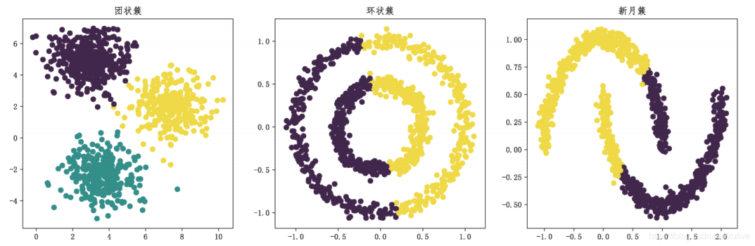
>>> from sklearn.cluster import KMeans # 从聚类子模块导入聚类模型>>> import matplotlib.pyplot as plt>>> plt.rcParams['font.sans-serif'] = ['FangSong']>>> plt.rcParams['axes.unicode_minus'] = False>>> X_blob, y_blob = dss.make_blobs(n_samples=[300,400,300], n_features=2)>>> X_circle, y_circle = dss.make_circles(n_samples=1000, noise=0.05, factor=0.5)>>> X_moon, y_moon = dss.make_moons(n_samples=1000, noise=0.05)>>> y_blob_pred = KMeans(init='k-means++', n_clusters=3).fit_predict(X_blob)>>> y_circle_pred = KMeans(init='k-means++', n_clusters=2).fit_predict(X_circle)>>> y_moon_pred = KMeans(init='k-means++', n_clusters=2).fit_predict(X_moon)>>> plt.subplot(131)<matplotlib.axes._subplots.AxesSubplot object at 0x00000180AFDECB88>>>> plt.title('团状簇')Text(0.5, 1.0, '团状簇')>>> plt.scatter(X_blob[:,0], X_blob[:,1], c=y_blob_pred)<matplotlib.collections.PathCollection object at 0x00000180C495DF08>>>> plt.subplot(132)<matplotlib.axes._subplots.AxesSubplot object at 0x00000180C493FA08>>>> plt.title('环状簇')Text(0.5, 1.0, '环状簇')>>> plt.scatter(X_circle[:,0], X_circle[:,1], c=y_circle_pred)<matplotlib.collections.PathCollection object at 0x00000180C499B888>>>> plt.subplot(133)<matplotlib.axes._subplots.AxesSubplot object at 0x00000180C4981188>>>> plt.title('新月簇')Text(0.5, 1.0, '新月簇')>>> plt.scatter(X_moon[:,0], X_moon[:,1], c=y_moon_pred)<matplotlib.collections.PathCollection object at 0x00000180C49DD1C8>>>> plt.show()

上面的代码首先使用样本生成器生成团状簇、环状簇和新月簇，然后使用k均值聚类分别对其实施聚类操作。结果表明，k均值聚类仅适用于团状簇，对于环状簇、新月簇无能为力。聚类的最终效果如下图所示。

基于密度的空间聚类具有更好的适应性，可以发现任何形状的簇。

基于密度的空间聚类，全称是基于密度的带噪声的空间聚类应用算法（英文简写为DBSCAN）。该聚类算法将簇视为被低密度区域分隔的高密度区域，这与K均值聚类假设簇总是凸的这一条件完全不同，因此可以发现任何形状的簇。

DBSCAN类是Scikit-learn聚类子模块cluster提供的基于密度的空间聚类算法，该类有两个重要参数eps和min_samples。要理解DBSCAN 类的参数，需要先理解核心样本。如果一个样本的eps距离范围内存在不少于min_sample个样本（包括这个样本），则该样本称为核心样本。可见，参数eps和min_samples 定义了簇的稠密度。

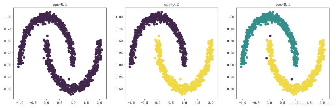
>>> from sklearn import datasets as dss>>> from sklearn.cluster import DBSCAN>>> import matplotlib.pyplot as plt>>> plt.rcParams['font.sans-serif'] = ['FangSong']>>> plt.rcParams['axes.unicode_minus'] = False>>> X, y = dss.make_moons(n_samples=1000, noise=0.05)>>> dbs_1 = DBSCAN() # 默认核心样本半径0.5，核心样本邻居5个>>> dbs_2 = DBSCAN(eps=0.2) # 核心样本半径0.2，核心样本邻居5个>>> dbs_3 = DBSCAN(eps=0.1) # 核心样本半径0.1，核心样本邻居5个>>> dbs_1.fit(X)DBSCAN(algorithm='auto', eps=0.5, leaf_size=30, metric='euclidean', metric_params=None, min_samples=5, n_jobs=None, p=None)>>> dbs_2.fit(X)DBSCAN(algorithm='auto', eps=0.2, leaf_size=30, metric='euclidean', metric_params=None, min_samples=5, n_jobs=None, p=None)>>> dbs_3.fit(X)DBSCAN(algorithm='auto', eps=0.1, leaf_size=30, metric='euclidean', metric_params=None, min_samples=5, n_jobs=None, p=None)>>> plt.subplot(131)<matplotlib.axes._subplots.AxesSubplot object at 0x00000180C4C5D708>>>> plt.title('eps=0.5')Text(0.5, 1.0, 'eps=0.5')>>> plt.scatter(X[:,0], X[:,1], c=dbs_1.labels_)<matplotlib.collections.PathCollection object at 0x00000180C4C46348>>>> plt.subplot(132)<matplotlib.axes._subplots.AxesSubplot object at 0x00000180C4C462C8>>>> plt.title('eps=0.2')Text(0.5, 1.0, 'eps=0.2')>>> plt.scatter(X[:,0], X[:,1], c=dbs_2.labels_)<matplotlib.collections.PathCollection object at 0x00000180C49FC8C8>>>> plt.subplot(133)<matplotlib.axes._subplots.AxesSubplot object at 0x00000180C49FCC08>>>> plt.title('eps=0.1')Text(0.5, 1.0, 'eps=0.1')>>> plt.scatter(X[:,0], X[:,1], c=dbs_3.labels_)<matplotlib.collections.PathCollection object at 0x00000180C49FC4C8>>>> plt.show()

以上代码使用DBSCAN，配合适当的参数，最终将新月数据集的上弦月和下弦月分开，效果如下图所示。

主成分分析（PCA）是一种统计方法，也是最常用的降维方法。

主成分分析通过正交变换将一组可能存在相关性的变量转换为一组线性不相关的变量，转换后的这组变量叫主成分。显然，主成分分析的降维并不是简单地丢掉一些特征，而是通过正交变换，把具有相关性的高维变量合并为线性无关的低维变量，从而达到降维的目的。

以下代码以鸢尾花数据集为例演示了如何使用 PCA 类来实现主成分分析和降维。已知鸢尾花数据集有 4 个特征列，分别是花萼的长度、宽度和花瓣的长度、宽度。

>>> from sklearn import datasets as dss>>> from sklearn.decomposition import PCA>>> ds = dss.load_iris()>>> ds.data.shape # 150个样本，4个特征维(150, 4)>>> m = PCA() # 使用默认参数实例化PCA类，n_components=None>>> m.fit(ds.data)PCA(copy=True, iterated_power='auto', n_components=None, random_state=None, svd_solver='auto', tol=0.0, whiten=False)>>> m.explained_variance_ # 正交变换后各成分的方差值array([4.22824171, 0.24267075, 0.0782095 , 0.02383509])>>> m.explained_variance_ratio_ # 正交变换后各成分的方差值占总方差值的比例array([0.92461872, 0.05306648, 0.01710261, 0.00521218])

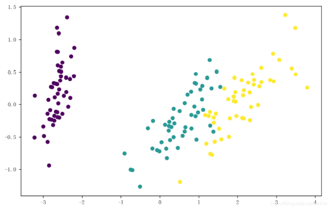
对鸢尾花数据集的主成分分析结果显示：存在一个明显的成分，其方差值占总方差值的比例超过92% ；存在一个方差值很小的成分，其方差值占总方差值的比例只有0.52% ；前两个成分贡献的方差占比超过97.7%，数据集特征列可以从4个降至2个而不至于损失太多有效信息。

>>> m = PCA(n_components=0.97)>>> m.fit(ds.data)PCA(copy=True, iterated_power='auto', n_components=0.97, random_state=None, svd_solver='auto', tol=0.0, whiten=False)>>> m.explained_variance_array([4.22824171, 0.24267075])>>> m.explained_variance_ratio_array([0.92461872, 0.05306648])>>> d = m.transform(ds.data)>>> d.shape(150, 2)

指定参数n_components不小于0.97，即可得到原数据集的降维结果：同样是150个样本，但特征列只有2个。若将2个特征列视为平面直角坐标系中的x和y坐标，就可以直观地画出全部样本数据。

>>> import matplotlib.pyplot as plt>>> plt.scatter(d[:,0], d[:,1], c=ds.target)<matplotlib.collections.PathCollection object at 0x0000016FBF243CC8>>>> plt.show()

下图显示只用2个特征维也基本可以分辨出鸢尾花的3种类型。

编辑：王菁

72张PNG，图解机器学习

PyTorch从入门到项目实践

PyTorch那些事儿（二）：PyTorch建模示例

PyTorch那些事儿（十三）：深度学习模型训练过程

PyTorch那些事儿（十四）：深度学习训练过程可视化

PyTorch那些事儿（十九）：深度学习实战项目——垃圾分类

可能是全网最全的速查表：Python机器学习ChatGPT线性代数微积分概率统计