
使用直方图处理进行颜色校正
点击上方“小白学视觉”,选择加"星标"或“置顶”
重磅干货,第一时间送达

在这篇文章中,我们将探讨如何使用直方图处理技术来校正图像中的颜色。
像往常一样,我们导入库,如numpy和matplotlib。此外,我们还从skimage 和scipy.stats库中导入特定函数。
import numpy as npimport matplotlib.pyplot as pltfrom skimage.io import imread, imshowfrom skimage import img_as_ubytefrom skimage.color import rgb2grayfrom skimage.exposure import histogram, cumulative_distributionfrom scipy.stats import cauchy, logistic
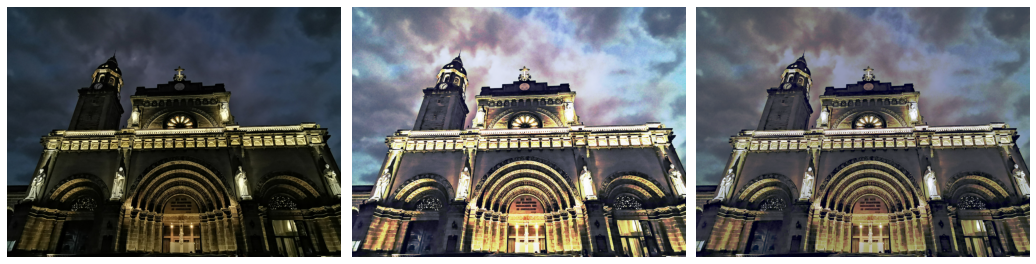
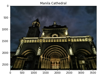
让我们使用马尼拉内穆罗斯马尼拉大教堂的夜间图像。
cathedral = imread('cathedral.jpg')plt.imshow(cathedral)plt.title('Manila Cathedral')
首先,让我们将图像转换为灰度。
fig, ax = plt.subplots(1,2, figsize=(15,5))cathedral_gray = rgb2gray(cathedral)ax[0].imshow(cathedral_gray, cmap='gray')ax[0].set_title('Grayscale Image')ax1 = ax[1]ax2 = ax1.twinx()freq_h, bins_h = histogram(cathedral_gray)freq_c, bins_c = cumulative_distribution(cathedral_gray)ax1.step(bins_h, freq_h*1.0/freq_h.sum(), c='b', label='PDF')ax2.step(bins_c, freq_c, c='r', label='CDF')ax1.set_ylabel('PDF', color='b')ax2.set_ylabel('CDF', color='r')ax[1].set_xlabel('Intensity value')ax[1].set_title('Histogram of Pixel Intensity');
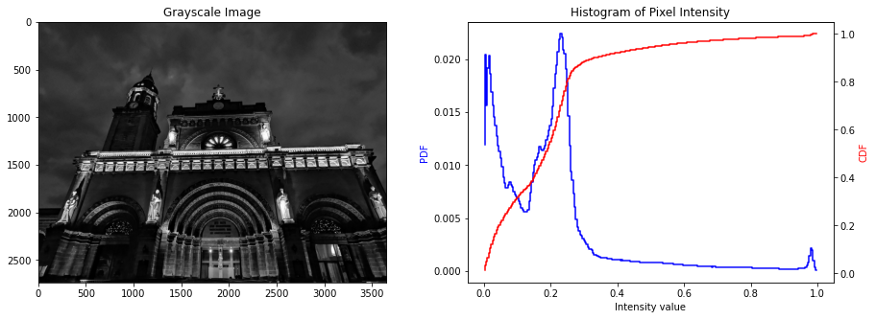
由于图像是在夜间拍摄的,因此图像的特征比较模糊,这也在像素强度值的直方图上观察到,其中 PDF 在较低的光谱上偏斜。
由于图像的强度值是倾斜的,因此可以应用直方图处理来重新分布图像的强度值。直方图处理的目的是将图像的实际 CDF 拉伸到新的目标 CDF 中。通过这样做,倾斜到较低光谱的强度值将转换为较高的强度值,从而使图像变亮。
让我们尝试在灰度图像上实现这一点,我们假设 PDF 是均匀分布,CDF 是线性分布。
image_intensity = img_as_ubyte(cathedral_gray)freq, bins = cumulative_distribution(image_intensity)target_bins = np.arange(255)target_freq = np.linspace(0, 1, len(target_bins))new_vals = np.interp(freq, target_freq, target_bins)fig, ax = plt.subplots(1,2, figsize=(15,5))ax[0].step(bins, freq, c='b', label='Actual CDF')ax[0].plot(target_bins, target_freq, c='r', label='Target CDF')ax[0].legend()ax[0].set_title('Grayscale: Actual vs. ''Target Cumulative Distribution')ax[1].imshow(new_vals[image_intensity].astype(np.uint8),cmap='gray')ax[1].set_title('Corrected Image in Grayscale');
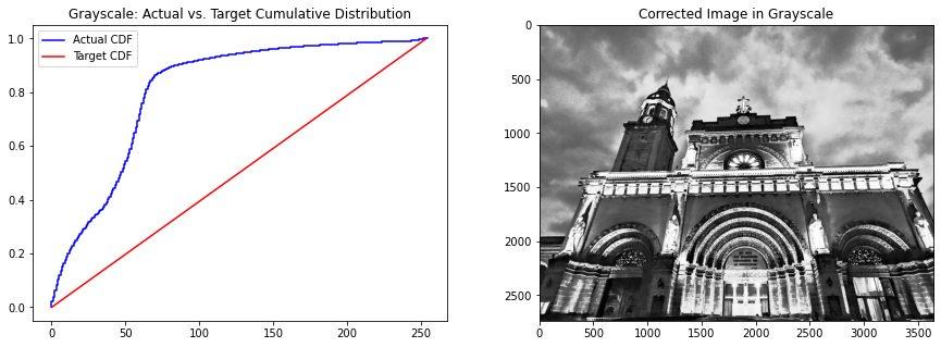
通过将实际 CDF 转换为目标 CDF,我们可以在保持图像关键特征的同时使图像变亮。请注意,这与仅应用亮度过滤器完全不同,因为亮度过滤器只是将图像中所有像素的强度值增加相等的量。在直方图处理中,像素强度值可以根据目标 CDF 增加或减少。
现在,让我们尝试在彩色图像中实现直方图处理。这些过程可以从灰度图像中复制——然而,不同之处在于我们需要对图像的每个通道应用直方图处理。为了简化实现,我们创建一个函数来对图像执行此过程。
def show_linear_cdf(image, channel, name, ax):image_intensity = img_as_ubyte(image[:,:,channel])freq, bins = cumulative_distribution(image_intensity)target_bins = np.arange(255)target_freq = np.linspace(0, 1, len(target_bins))ax.step(bins, freq, c='b', label='Actual CDF')ax.plot(target_bins, target_freq, c='r', label='Target CDF')ax.legend()ax.set_title('{} Channel: Actual vs. ''Target Cumulative Distribution'.format(name))def linear_distribution(image, channel):image_intensity = img_as_ubyte(image[:,:,channel])freq, bins = cumulative_distribution(image_intensity)target_bins = np.arange(255)target_freq = np.linspace(0, 1, len(target_bins))new_vals = np.interp(freq, target_freq, target_bins)return new_vals[image_intensity].astype(np.uint8)
现在,我们将这些函数应用于原始图像的每个通道。
fig, ax = plt.subplots(3,2, figsize=(12,14))red_channel = linear_distribution(cathedral, 0)green_channel = linear_distribution(cathedral, 1)blue_channel = linear_distribution(cathedral, 2)show_linear_cdf(cathedral, 0, ‘Red’, ax[0,0])ax[0,1].imshow(red_channel, cmap=’Reds’)ax[0,1].set_title(‘Corrected Image in Red Channel’)show_linear_cdf(cathedral, 1, ‘Green’, ax[1,0])ax[1,1].imshow(green_channel, cmap=’Greens’)ax[1,1].set_title(‘Corrected Image in Green Channel’)show_linear_cdf(cathedral, 2, ‘Blue’, ax[2,0])ax[2,1].imshow(blue_channel, cmap=’Blues’)ax[2,1].set_title(‘Corrected Image in Blue Channel’)
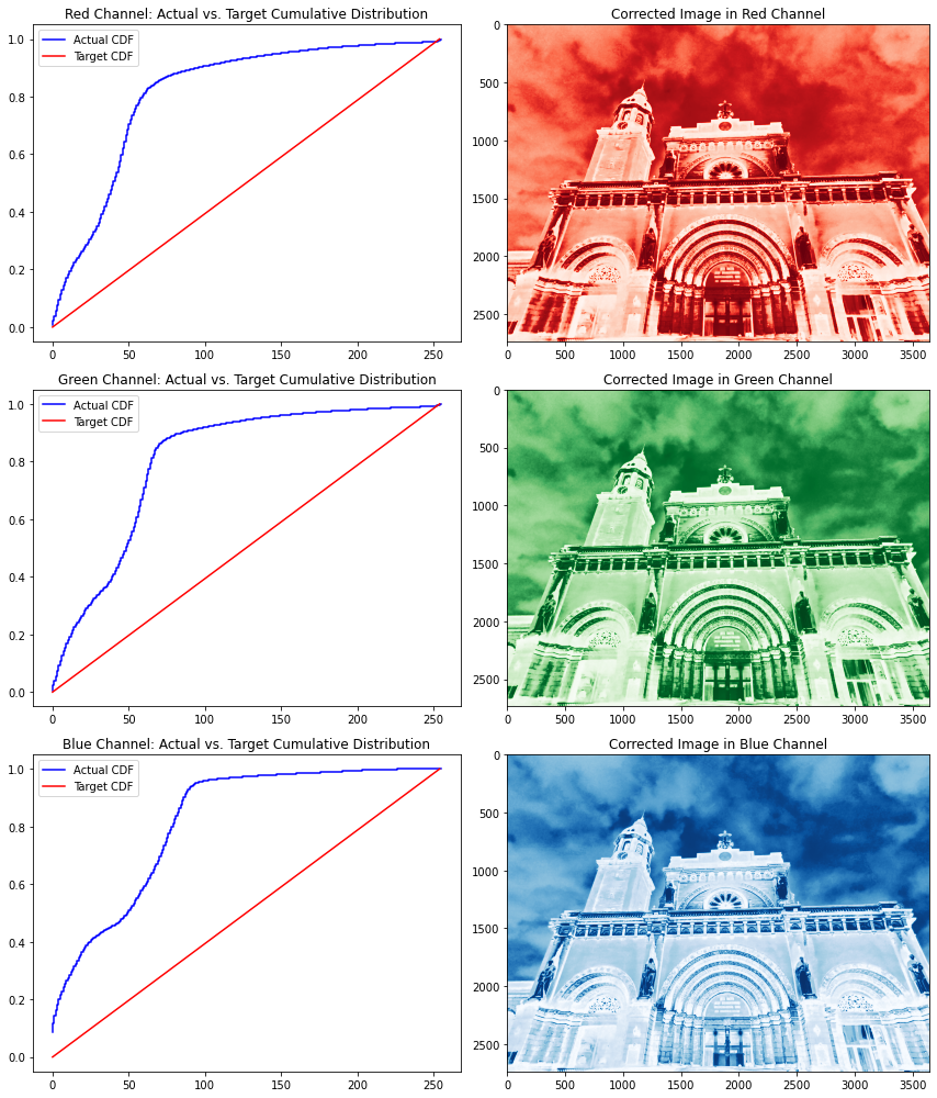
请注意,所有通道几乎都具有相同的 CDF,这显示了图像中颜色的良好分布——只是颜色集中在较低的强度值光谱上。就像我们在灰度图像中所做的一样,我们还将每个通道的实际 CDF 转换为目标 CDF。
校正每个通道的直方图后,我们需要使用 numpy stack函数将这些通道堆叠在一起。请注意,RGB 通道在堆叠时需要按顺序排列。
fig, ax = plt.subplots(1,2, figsize=(15,5))ax[0].imshow(cathedral);ax[0].set_title('Original Image')ax[1].imshow(np.dstack([red_channel, green_channel, blue_channel]));ax[1].set_title('Transformed Image');
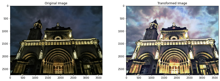
堆叠所有通道后,我们可以看到转换后的图像颜色与原始图像的显着差异。直方图处理最有趣的地方在于,图像的不同部分会有不同程度的像素强度转换。请注意,马尼拉大教堂墙壁的像素强度发生了巨大变化,而马尼拉大教堂钟楼的像素强度却保持相对不变。
现在,让我们尝试使用其他函数作为目标 CDF 来改进这一点。为此,我们将使用该scipy.stats库导入各种分布,还创建了一个函数来简化我们的分析。
def individual_channel(image, dist, channel):im_channel = img_as_ubyte(image[:,:,channel])freq, bins = cumulative_distribution(im_channel)new_vals = np.interp(freq, dist.cdf(np.arange(0,256)),np.arange(0,256))return new_vals[im_channel].astype(np.uint8)def distribution(image, function, mean, std):dist = function(mean, std)fig, ax = plt.subplots(1,2, figsize=(15,5))image_intensity = img_as_ubyte(rgb2gray(image))freq, bins = cumulative_distribution(image_intensity)ax[0].step(bins, freq, c='b', label='Actual CDF')ax[0].plot(dist.cdf(np.arange(0,256)),c='r', label='Target CDF')ax[0].legend()ax[0].set_title('Actual vs. Target Cumulative Distribution')red = individual_channel(image, dist, 0)green = individual_channel(image, dist, 1)blue = individual_channel(image, dist, 2)ax[1].imshow(np.dstack((red, green, blue)))ax[1].set_title('Transformed Image')return ax
让我们使用 Cauchy 函数来试试这个。
distribution(cathedral, cauchy, 90, 30);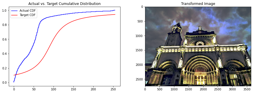
使用不同的分布似乎会产生更令人愉悦的配色方案。事实上,大教堂正门的弧线在逻辑分布中比线性分布更好,这是因为在逻辑分布中像素值强度的平移比线性分布要小,这可以从实际 CDF 线到目标 CDF 线的距离看出。
让我们看看我们是否可以使用逻辑分布进一步改进这一点。
distribution(cathedral, logistic, 90, 30);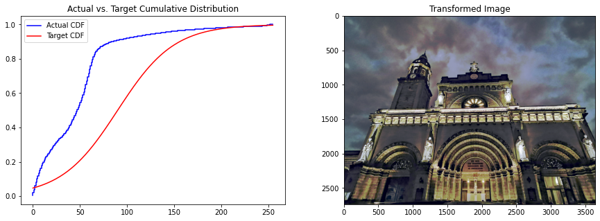
请注意,门中的灯光如何从线性和Cauchy分布改进为逻辑分布的。这是因为逻辑函数的上谱几乎与原始 CDF 一致。因此,图像中的所有暗物体(低像素强度值)都被平移,而灯光(高像素强度值)几乎保持不变。
我们已经探索了如何使用直方图处理来校正图像中的颜色,实现了各种分布函数,以了解它如何影响结果图像中的颜色分布。
同样,我们可以得出结论,在固定图像的颜色强度方面没有“一体适用”的解决方案,数据科学家的主观决定是确定哪个是最适合他们的图像处理需求的解决方案。
Github代码连接:
https://github.com/jephraim-manansala/histogram-manipulation
交流群
欢迎加入公众号读者群一起和同行交流,目前有SLAM、三维视觉、传感器、自动驾驶、计算摄影、检测、分割、识别、医学影像、GAN、算法竞赛等微信群(以后会逐渐细分),请扫描下面微信号加群,备注:”昵称+学校/公司+研究方向“,例如:”张三 + 上海交大 + 视觉SLAM“。请按照格式备注,否则不予通过。添加成功后会根据研究方向邀请进入相关微信群。请勿在群内发送广告,否则会请出群,谢谢理解~