
机器学习:从零开始学习梯度下降
作者:SETHNEHA 翻译:王可汗 校对:陈丹
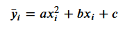
coeffs = [2,-5, 4]def eval_2nd_degree(coeffs, x):"""Function to return the outputof evaluating a second degree polynomial,given a specific x value.Args:coeffs: List containingthe coefficients a,b, and c for the polynomial.x: The input x value tothe polynomial.Returns:y: The correspondingoutput y value for the second degree polynomial."""a = (coeffs[0]*(x*x))b = coeffs[1]*xc = coeffs[2]y = a+b+creturn y
coeffs = [2, -5, 4]x=3eval_2nd_degree(coeffs, x)7
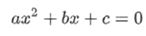
import numpy as npimport matplotlib.pyplot as plthundred_xs=np.random.uniform(-10,10,100)print(hundred_xs)x_y_pairs = []for x in hundred_xs:y =eval_2nd_degree(coeffs, x)x_y_pairs.append((x,y))xs = []ys = []for a,b in x_y_pairs:xs.append(a)ys.append(b)plt.figure(figsize=(20,10))plt.plot(xs, ys, 'g+')plt.title('Original data')plt.show()
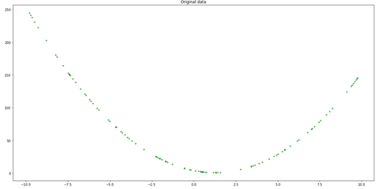
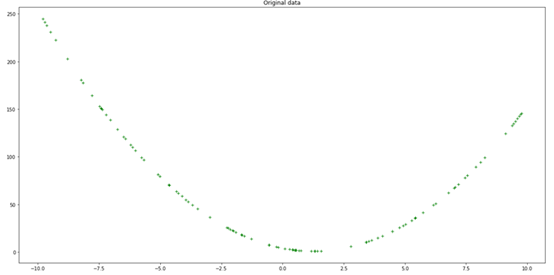
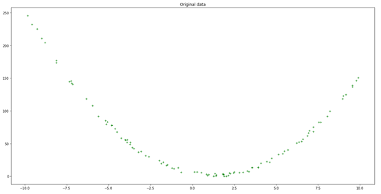
defeval_2nd_degree_jitter(coeffs, x, j):"""Function to return the noisy output ofevaluating a second degree polynomial,given a specific x value. Output values canbe within [y−j,y+j].Args:coeffs: List containing thecoefficients a,b, and c for the polynomial.x: The input x value to the polynomial.j: Jitter parameter, to introduce noiseto output y.Returns:y: The corresponding jittered output yvalue for the second degree polynomial."""a = (coeffs[0]*(x*x))b = coeffs[1]*xc = coeffs[2]y = a+b+cprint(y)interval = [y-j, y+j]interval_min = interval[0]interval_max = interval[1]print(f"Should get value in the range{interval_min} - {interval_max}")jit_val = random.random() *interval_max # Generate a randomnumber in range 0 to interval maxwhile interval_min > jit_val: # While the random jittervalue is less than the interval min,jit_val = random.random() *interval_max # it is not in the rightrange. Re-roll the generator until it# give a number greater than the interval min.return jit_val
7Should get value in the range 3 - 116.233537936801398
x_y_pairs = []for x in hundred_xs:y =eval_2nd_degree_jitter(coeffs, x, j)x_y_pairs.append((x,y))xs = []ys = []for a,b in x_y_pairs:xs.append(a)ys.append(b)plt.figure(figsize=(20,10))plt.plot(xs, ys, 'g+')plt.title('Original data')plt.show()
rand_coeffs=(random.randrange(-10,10),random.randrange(-10,10),random.randrange(-10,10))rand_coeffs(7, 6, 3)
y_bar =eval_2nd_degree(rand_coeffs, hundred_xs)plt.figure(figsize=(20,10))plt.plot(xs, ys, 'g+', label ='original')plt.plot(xs, y_bar, 'ro',label='prediction')plt.title('Original data vsfirst prediction')plt.legend(loc="lowerright")plt.show()
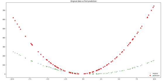
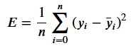
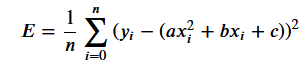
def loss_mse(ys, y_bar):"""Calculates MSE loss.Args:ys: training data labelsy_bar: prediction labelsReturns: Calculated MSE loss."""return sum((ys - y_bar)*(ys - y_bar)) /len(ys)initial_model_loss = loss_mse(ys, y_bar)initial_model_loss47922.39790821987
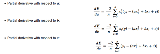
如果你计算每个导数的值,你会得到每个系数的梯度。 这些值给出了损失函数相对于每个特定系数的斜率。 它们表明你应该增加还是减少它来减少损失,以及这样做的安全程度。
defcalc_gradient_2nd_poly(rand_coeffs, hundred_xs, ys):"""calculates the gradient for a second degreepolynomial.Args:coeffs: a,b and c, for a 2nd degreepolynomial [ y = ax^2 + bx + c ]inputs_x: x input datapointsoutputs_y: actual y output pointsReturns: Calculated gradients for the 2nddegree polynomial, as a tuple of its parts for a,b,c respectively."""a_s = []b_s = []c_s = []y_bars = eval_2nd_degree(rand_coeffs,hundred_xs)for x,y,y_bar in list(zip(hundred_xs, ys,y_bars)): # take tuple of (xdatapoint, actual y label, predicted y label)x_squared = x**2partial_a = x_squared * (y - y_bar)a_s.append(partial_a)partial_b = x * (y-y_bar)b_s.append(partial_b)partial_c = (y-y_bar)c_s.append(partial_c)num = [i for i in y_bars]n = len(num)gradient_a = (-2 / n) * sum(a_s)gradient_b = (-2 / n) * sum(b_s)gradient_c = (-2 / n) * sum(c_s)return(gradient_a, gradient_b,gradient_c) # return calculatedgradients as a a tuple of its 3 parts
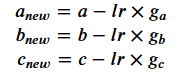
使用上面的函数来计算我们表现不佳的随机模型的梯度。 相应调整模型系数。 验证模型的损失现在更小了——梯度下降起作用了!
calc_grad= calc_gradient_2nd_poly(rand_coeffs, hundred_xs, ys)lr =0.0001a_new= rand_coeffs[0] - lr * calc_grad[0]b_new= rand_coeffs[1] - lr * calc_grad[1]c_new= rand_coeffs[2] - lr * calc_grad[2]new_model_coeffs= (a_new, b_new, c_new)print(f"Newmodel coeffs: {new_model_coeffs}")print("")#updatewith these new coeffs:new_y_bar= eval_2nd_degree(new_model_coeffs, hundred_xs)updated_model_loss= loss_mse(ys, new_y_bar)print(f"Nowhave smaller model loss: {updated_model_loss} vs {original_model_loss}")
New model coeffs: 5.290395171471687 5.903335222089396 2.9704266522693037Now have smaller model loss: 23402.14716735533 vs 47922.39790821987
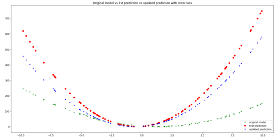
plt.figure(figsize=(20,10))plt.plot(xs, ys, 'g+', label ='original model')plt.plot(xs, y_bar, 'ro', label= 'first prediction')plt.plot(xs, new_y_bar, 'b.',label = 'updated prediction')plt.title('Original model vs1st prediction vs updated prediction with lower loss')plt.legend(loc="lower right")plt.show()
defcalc_gradient_2nd_poly_for_GD(coeffs, inputs_x, outputs_y, lr):"""calculates the gradient for a second degreepolynomial.Args:coeffs: a,b and c, for a 2nd degreepolynomial [ y = ax^2 + bx + c ]inputs_x: x input datapointsoutputs_y: actual y output pointslr: learning rateReturns: Calculated gradients for the 2nddegree polynomial, as a tuple of its parts for a,b,c respectively."""a_s = []b_s = []c_s = []y_bars = eval_2nd_degree(coeffs, inputs_x)for x,y,y_bar in list(zip(inputs_x,outputs_y, y_bars)): # take tuple of(x datapoint, actual y label, predicted y label)x_squared = x**2partial_a = x_squared * (y - y_bar)a_s.append(partial_a)partial_b = x * (y-y_bar)b_s.append(partial_b)partial_c = (y-y_bar)c_s.append(partial_c)num = [i for i in y_bars]n = len(num)gradient_a = (-2 / n) * sum(a_s)gradient_b = (-2 / n) * sum(b_s)gradient_c = (-2 / n) * sum(c_s)a_new = coeffs[0] - lr * gradient_ab_new = coeffs[1] - lr * gradient_bc_new = coeffs[2] - lr * gradient_cnew_model_coeffs = (a_new, b_new, c_new)#update with these new coeffs:new_y_bar = eval_2nd_degree(new_model_coeffs,inputs_x)updated_model_loss = loss_mse(outputs_y,new_y_bar)return updated_model_loss,new_model_coeffs, new_y_bar
def gradient_descent(epochs,lr):"""Perform gradient descent for a seconddegree polynomial.Args:epochs: number of iterations to performof finding new coefficients and updatingt loss.lr: specified learning rateReturns: Tuple containing (updated_model_loss,new_model_coeffs, new_y_bar predictions, saved loss updates)"""losses = []rand_coeffs_to_test = rand_coeffsfor i in range(epochs):loss =calc_gradient_2nd_poly_for_GD(rand_coeffs_to_test, hundred_xs, ys, lr)rand_coeffs_to_test = loss[1]losses.append(loss[0])print(losses)return loss[0], loss[1], loss[2],losses #(updated_model_loss,new_model_coeffs, new_y_bar, saved loss updates)
GD = gradient_descent(1500,0.0001)plt.figure(figsize=(20,10))plt.plot(xs, ys, 'g+', label ='original')plt.plot(xs, GD[2], 'b.', label= 'final_prediction')plt.title('Original vs Finalprediction after Gradient Descent')plt.legend(loc="lowerright")plt.show()
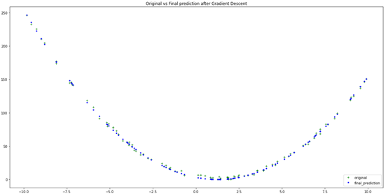
print(f"FinalCoefficients predicted: {GD[1]}")print(f"OriginalCoefficients: {coeffs}")
Final Coefficients predicted: (2.0133237089326155, -4.9936501002139275, 3.1596042252126195)Original Coefficients: [2, -5, 4]
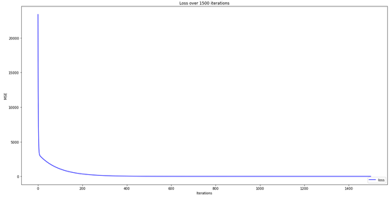
plt.figure(figsize=(20,10))plt.plot(GD[3], 'b-', label ='loss')plt.title('Loss over 1500iterations')plt.legend(loc="lowerright")plt.xlabel('Iterations')plt.ylabel('MSE')plt.show()
也可以加一下老胡的微信 围观朋友圈~~~
推荐阅读
(点击标题可跳转阅读)
麻省理工学院计算机课程【中文版】 【清华大学王东老师】现代机器学习技术导论.pdf 机器学习中令你事半功倍的pipeline处理机制 机器学习避坑指南:训练集/测试集分布一致性检查 机器学习深度研究:特征选择中几个重要的统计学概念 老铁,三连支持一下,好吗?↓↓↓
评论