基于CNN的图像缺陷分类

点击上方“小白学视觉”，选择加"星标"或“置顶”

重磅干货，第一时间送达

本文转自|新机器视觉

来源：博客园  原文地址：https://www.cnblogs.com/BellaVita/p/10142266.html

1、前言　　

在工业产品缺陷检测中，基于传统的图像特征的缺陷分类的准确率达不到实际生产的要求，因此想采用CNN来进行缺陷分类。

　　传统缺陷分类思路：

　　1、缺陷图片分离：先采用复杂的图像处理方法，将缺陷从采集的图像中分离处理；

　　2、特征向量构建：通过对不同缺陷种类的特征进行分析，定义需要提取的n维特征（比如缺陷长、宽、对比度、纹理特征、熵、梯度等），构成一组描述缺陷的

　　　　　　　　　　  特征向量；特征向量的构建需要对实际的问题有很深入的分析，并且需要有很深厚的图像处理知识；这也是传统分类问题中最难的部分。

　　3、特征向量归一化：由于特征向量每个维度的度量差别很大（比如缺陷长50像素，对比度0.03），因此需要进行特征缩放，特征归一化；

　　4、人工标记缺陷：将缺陷图片存储在人工标记的文件夹内；

　　5、采用SVM对缺陷进行分类，分类准确率85%左右。

2、CNN网络构建

　　在缺陷图片分离和人工标记后，构建CNN网络模型；由于工业检测中对实时性要求很高，因此想采用比较简单的网络结构来提高训练的速度和检测速度；

　　网络构建：本文采用LeNet网络结构的基本思路，构建一个简单的网络

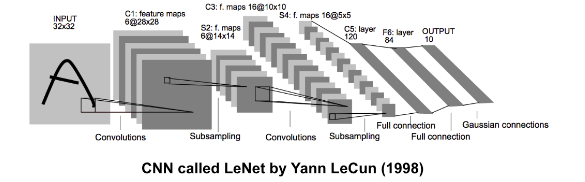
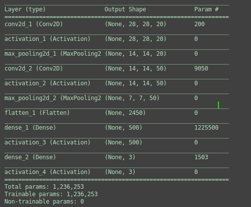
图1：Tensorflow输出的网络模型

3、模型训练和测试

3.1 原始模型测试

　　开始以为模型可能会出现过拟合的问题，不过从精度和损失曲线看来，没有过拟合问题，到是模型初始迭代的时候陷入了一个局部循环状态，可能是没有得到特别好的特征或者是随机选择训练模型的数据集没有完全分散，也有可能是训练的次数太少了。训练集上的准确率有点低，因此需要用更好的模型，但是模型怎么改呢？？尽管CNN可以自己训练出FIlters，但是依然不能很清晰的看到图像被滤波后是怎么样的状态（图2,图3），对于一直做图像底层算法的人来说，有点很不爽。

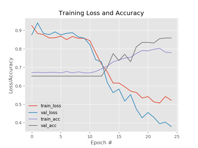
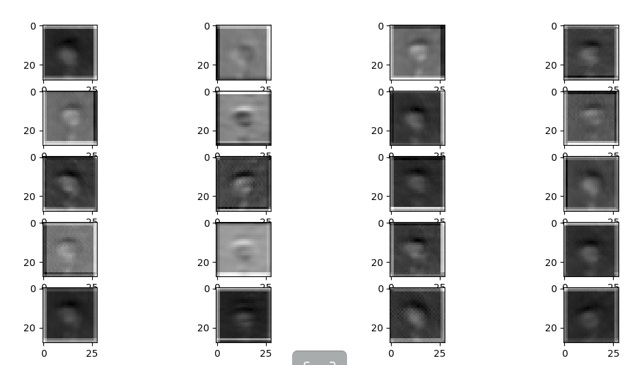
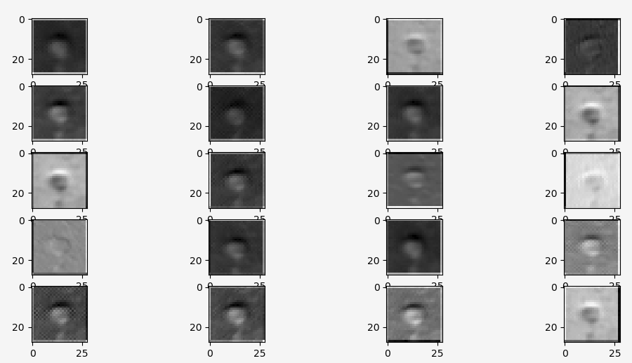
图2 ：卷积第一层

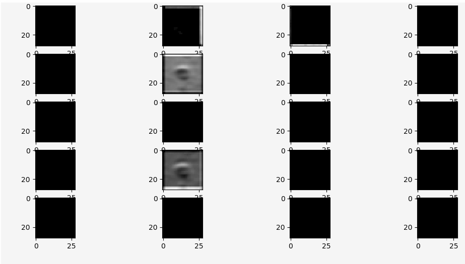
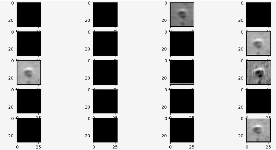
图3：Relu激活函数层

　　通过分析图2，发现滤波整体效果还不错，缺陷的地方都能清晰的反映出来；但是本来输入的缺陷是往下凹的，滤波后的缺陷很多是向上凸的，不符合实际情况。

　　分析图3,发现经过Relu激活函数后，只留下了很明显向下凹的缺陷特征图片，但是有效的特征图片（FeatureMap）太少，只有2个。

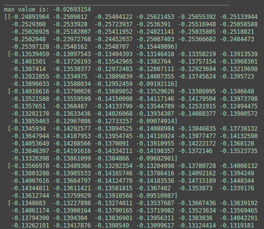
图4：上凸图片数据

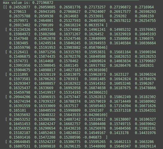
图5：下凹图片数据

　　为了能得到更多的符合实际的缺陷特征图片，考虑到需要更加突出缺陷边缘，以致不被周围大片图像的干扰，因此决定将卷积核变小；卷积核由默认的5x5改为3x3.

3.2 优化卷积核大小后

　　模型整体的精度有明显的上升，经过Relu后的有效FeatureMap增加了。有点疑问的是validation数据集的准确率比训练还高5-8个点？？？

4、Code

# -*- coding: utf-8 -*-
# @Time    : 18-7-25 下午2:33
# @Author  : DuanBin
# @Email   : 20092758@cqu.edu.cn
# @File    : catl_train.py
# @Software: PyCharm

# USAGE
# python catl_train.py --dataset data --model catl.model

# import the necessary packages
from keras.preprocessing.image import ImageDataGenerator
from keras.optimizers import Adam
from sklearn.model_selection import train_test_split
from keras.preprocessing.image import img_to_array
from keras.utils import to_categorical
from keras.models import Model
from keras.models import load_model
from lenet import LeNet
from imutils import paths
import matplotlib.pyplot as plt
import numpy as np
import argparse
import random
import cv2
import os

# set the matplotlib backend so figures can be saved in the background
import matplotlib
matplotlib.use("Agg")

dataPath = "data"
modelPath = "catl_5_5.model"
plotPath = "catl_plot_5_5_blog.png"

# initialize the number of epochs to train for, initia learning rate,
# and batch size
EPOCHS = 50
INIT_LR = 0.001
BS = 3
classNumber = 3
imageDepth = 1

# initialize the data and labels
print("[INFO] loading images...")
data = []
labels = []

# grab the image paths and randomly shuffle them
imagePaths = sorted(list(paths.list_images(dataPath)))  # args["dataset"])))
random.seed(42)
random.shuffle(imagePaths)

# loop over the input images
for imagePath in imagePaths:
    # load the image, pre-process it, and store it in the data list
    image = cv2.imread(imagePath, 0)
    image = cv2.resize(image, (28, 28))
    image = img_to_array(image)
    data.append(image)

    # extract the class label from the image path and update the
    # labels list
    label = imagePath.split(os.path.sep)[-2]
    if label == "dity":
        label = 0
    elif label == "tan":
        label = 1
    elif label == "valley":
        label = 2
    labels.append(label)

# scale the raw pixel intensities to the range [0, 1]
data = np.array(data, dtype="float") / 255.0
labels = np.array(labels)

# partition the data into training and testing splits using 75% of
# the data for training and the remaining 25% for testing
(trainX, testX, trainY, testY) = train_test_split(data, labels, test_size=0.3, random_state=42)
print(trainX.shape)

# convert the labels from integers to vectors
trainY = to_categorical(trainY, num_classes=classNumber)
testY = to_categorical(testY, num_classes=classNumber)
print(trainY.shape)
print(testX.shape)


# construct the image generator for data augmentation
aug = ImageDataGenerator(rotation_range=30, width_shift_range=0.1,
                         height_shift_range=0.1, shear_range=0.2, zoom_range=0.2,
                         horizontal_flip=True, fill_mode="nearest")

# # initialize the model
print("[INFO] compiling model...")
model = LeNet.build(width=28, height=28, depth=imageDepth, classes=classNumber)
opt = Adam(lr=INIT_LR, decay=INIT_LR / EPOCHS)
model.compile(loss="categorical_crossentropy", optimizer=opt,
              metrics=["accuracy"])

model.summary()

# train the network
print("[INFO] training network...")
H = model.fit_generator(aug.flow(trainX, trainY, batch_size=BS),
                        validation_data=(testX, testY), steps_per_epoch=len(trainX) // BS,
                        epochs=EPOCHS, verbose=1)

# save the model to disk
print("[INFO] serializing network...")
model.save(modelPath)  # args["model"])
model.save_weights("catl_5_5_wight.h5")

# plot the training loss and accuracy
plt.style.use("ggplot")
plt.figure()
N = EPOCHS
plt.plot(np.arange(0, N), H.history["loss"], label="train_loss")
plt.plot(np.arange(0, N), H.history["val_loss"], label="val_loss")
plt.plot(np.arange(0, N), H.history["acc"], label="train_acc")
plt.plot(np.arange(0, N), H.history["val_acc"], label="val_acc")
plt.title("Training Loss and Accuracy")
plt.xlabel("Epoch #")
plt.ylabel("Loss/Accuracy")
plt.legend(loc="lower left")
plt.savefig(plotPath)  # args["plot"])
plt.show()

layer_outputs = [layer.output for layer in model.layers]
activation_model = Model(inputs=model.input, outputs=layer_outputs)
activations = activation_model.predict(testX[0].reshape(1, 28, 28, 1))


def display_activation(activations, col_size, row_size, act_index):
    activation = activations[act_index]
    activation_index = 0
    fig, ax = plt.subplots(row_size, col_size, figsize=(row_size * 2.5, col_size * 1.5))
    for row in range(0, row_size):
        for col in range(0, col_size):
            ax[row][col].imshow(activation[0, :, :, activation_index], cmap='gray')
            activation_index += 1

    plt.show()


display_activation(activations, 4, 5, 1)

# import the necessary packages
from keras.models import Sequential
from keras.layers.convolutional import Conv2D
from keras.layers.convolutional import MaxPooling2D
from keras.layers.core import Activation
from keras.layers.core import Flatten
from keras.layers.core import Dense
from keras.layers.core import Dropout
from tensorflow.keras import backend as K


class LeNet:
    @staticmethod
    def build(width, height, depth, classes):
        # initialize the model
        model = Sequential()
        inputShape = (height, width, depth)

        # if we are using "channels first", update the input shape
        if K.image_data_format() == "channels_first":
            inputShape = (depth, height, width)
        else:
            inputShape = (width, height, depth)

        # first set of CONV => RELU => POOL layers
        model.add(Conv2D(20, (3, 3), padding="same", input_shape=inputShape))
        model.add(Activation("relu"))
        model.add(MaxPooling2D(pool_size=(2, 2), strides=(2, 2)))

        # second set of CONV => RELU => POOL layers
        model.add(Conv2D(50, (3, 3), padding="same"))
        model.add(Activation("relu"))
        model.add(MaxPooling2D(pool_size=(2, 2), strides=(2, 2)))


        # first (and only) set of FC => RELU layers
        model.add(Flatten())
        model.add(Dense(500))
        model.add(Activation("relu"))

        # softmax classifier
        model.add(Dense(classes))
        model.add(Activation("softmax"))

        # return the constructed network architecture
        return model

 End 

交流群

欢迎加入公众号读者群一起和同行交流，目前有SLAM、三维视觉、传感器、自动驾驶、计算摄影、检测、分割、识别、医学影像、GAN、算法竞赛等微信群（以后会逐渐细分），请扫描下面微信号加群，备注：”昵称+学校/公司+研究方向“，例如：”张三 + 上海交大 + 视觉SLAM“。请按照格式备注，否则不予通过。添加成功后会根据研究方向邀请进入相关微信群。请勿在群内发送广告，否则会请出群，谢谢理解~