
特殊图像的色彩特征工程:非自然图像的颜色编码

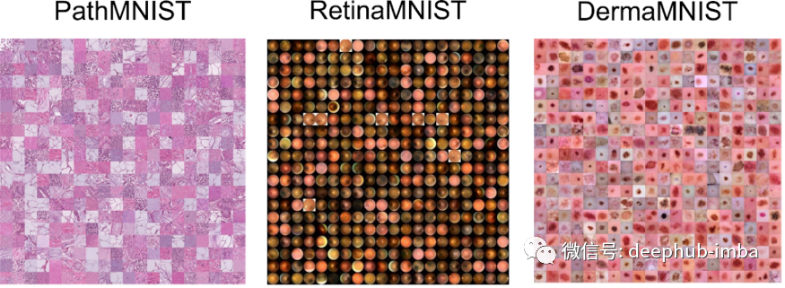
来源:DeepHub IMBA 本文共7500字,建议阅读15+分钟 我们将探讨特征工程的不同方式如何有助于提高卷积神经网络的分类性能。
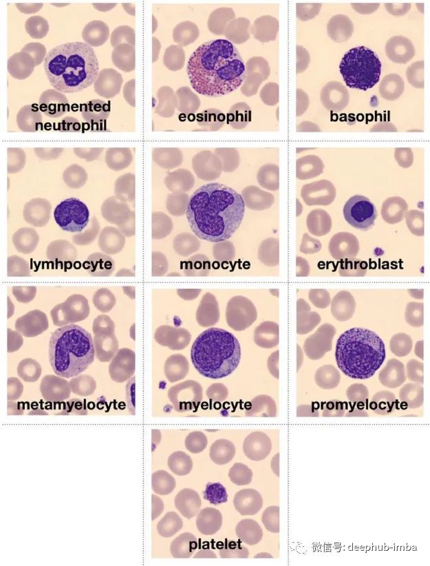
数据集
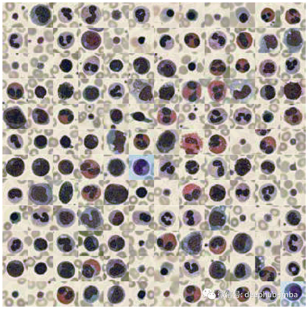
# Download dataset!wget https://zenodo.org/record/5208230/files/bloodmnist.npz# Load packagesimport numpy as npfrom glob import globimport matplotlib.pyplot as pltfrom tqdm.notebook import tqdmimport pandas as pdimport seaborn as snssns.set_context("talk")%config InlineBackend.figure_format = 'retina'# Load data setdata = np.load("bloodmnist.npz")X_tr = data["train_images"].astype("float32") / 255X_va = data["val_images"].astype("float32") / 255X_te = data["test_images"].astype("float32") / 255y_tr = data["train_labels"]y_va = data["val_labels"]y_te = data["test_labels"]labels = ["basophils", "eosinophils", "erythroblasts","granulocytes_immature", "lymphocytes","monocytes", "neutrophils", "platelets"]labels_tr = np.array([labels[j] for j in y_tr.ravel()])labels_va = np.array([labels[j] for j in y_va.ravel()])labels_te = np.array([labels[j] for j in y_te.ravel()])
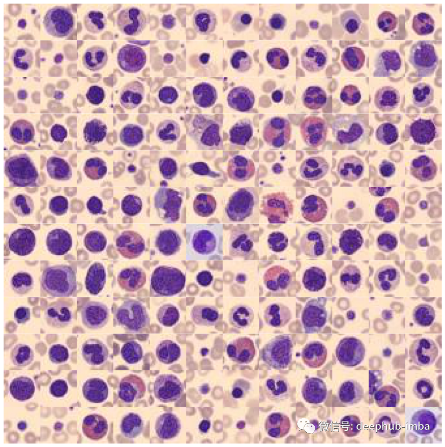
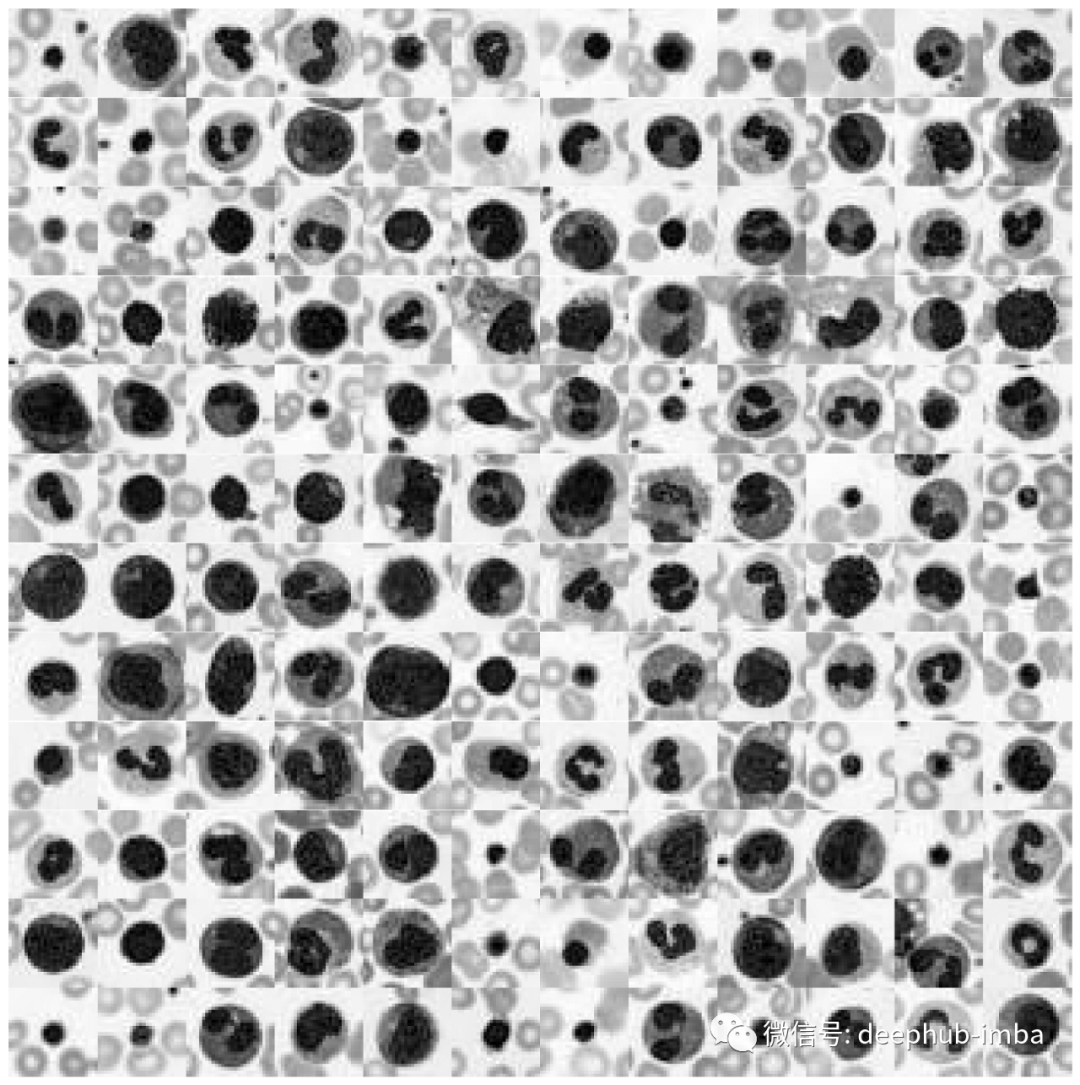
def plot_dataset(X):"""Helper function to visualize first few images of a dataset."""fig, axes = plt.subplots(12, 12, figsize=(15.5, 16))for i, ax in enumerate(axes.flatten()):if X.shape[-1] == 1:ax.imshow(np.squeeze(X[i]), cmap="gray")else:ax.imshow(X[i])ax.axis("off")ax.set_aspect("equal")plt.subplots_adjust(wspace=0, hspace=0)plt.show()# Plot datasetplot_dataset(X_tr)
# Extract a few RGB color valuesX_colors = X_tr.reshape(-1, 3)[::100]# Plot color values in 3D spacefig = plt.figure(figsize=(16, 5))# Loop through 3 different viewsfor i, view in enumerate([[-45, 10], [40, 80], [60, 10]]):ax = fig.add_subplot(1, 3, i + 1, projection="3d")ax.scatter(X_colors[:, 0], X_colors[:, 1], X_colors[:, 2], facecolors=X_colors, s=2)ax.set_xlabel("R")ax.set_ylabel("G")ax.set_zlabel("B")ax.xaxis.set_ticklabels([])ax.yaxis.set_ticklabels([])ax.zaxis.set_ticklabels([])ax.view_init(azim=view[0], elev=view[1], vertical_axis="z")ax.set_xlim(0, 1)ax.set_ylim(0, 1)ax.set_zlim(0, 1)plt.suptitle("Colors in RGB space", fontsize=20)plt.show()
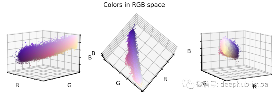
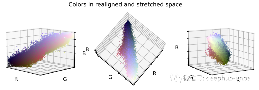
我们可以通过将 RGB 颜色转换为灰度图像来降低图像复杂性。 我们可以重新对齐和拉伸颜色值,以便 RGB 值更好地填充 RGB 颜色空间。 我们可以重新调整颜色值的方向,使三个立方体轴延伸到最大方差的方向。这最好通过 PCA 方法完成。
数据集扩充
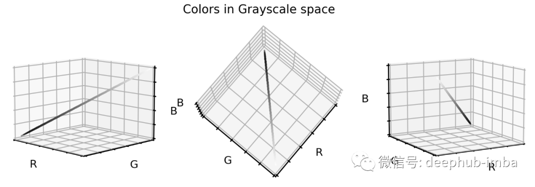
# Install scikit-image if not already done!pip install -U scikit-imagefrom skimage.color import rgb2gray# Create grayscale imagesX_tr_gray = rgb2gray(X_tr)[..., None]X_va_gray = rgb2gray(X_va)[..., None]X_te_gray = rgb2gray(X_te)[..., None]# Stretch color range to training min, maxgmin_tr = X_tr_gray.min()X_tr_gray -= gmin_trX_va_gray -= gmin_trX_te_gray -= gmin_trgmax_tr = X_tr_gray.max()X_tr_gray /= gmax_trX_va_gray /= gmax_trX_te_gray /= gmax_trX_va_gray = np.clip(X_va_gray, 0, 1)X_te_gray = np.clip(X_te_gray, 0, 1)让我们看看这些灰度颜色值是如何在之前的 RGB 颜色空间中定位的。# Put 1D values into 3D spaceX_tr_show = np.concatenate([X_tr_gray, X_tr_gray, X_tr_gray], axis=-1)# Extract a few grayscale color valuesX_grays = X_tr_show.reshape(-1, 3)[::100]# Plot color values in 3D spacefig = plt.figure(figsize=(16, 5))# Loop through 3 different viewsfor i, view in enumerate([[-45, 10], [40, 80], [60, 10]]):ax = fig.add_subplot(1, 3, i + 1, projection="3d")ax.scatter(X_grays[:, 0], X_grays[:, 1], X_grays[:, 2], facecolors=X_grays, s=2)ax.set_xlabel("R")ax.set_ylabel("G")ax.set_zlabel("B")ax.xaxis.set_ticklabels([])ax.yaxis.set_ticklabels([])ax.zaxis.set_ticklabels([])ax.view_init(azim=view[0], elev=view[1], vertical_axis="z")ax.set_xlim(0, 1)ax.set_ylim(0, 1)ax.set_zlim(0, 1)plt.suptitle("Colors in Grayscale space", fontsize=20)plt.show()
# Plot datasetplot_dataset(X_tr_gray)
# Get RGB color valuesX_colors = X_tr.reshape(-1, 3)# Get distance of all color values to black (0,0,0)dist_origin = np.linalg.norm(X_colors, axis=-1)# Find index of 0.1% smallest entryperc_sorted = np.argsort(np.abs(dist_origin - np.percentile(dist_origin, 0.1)))# Find centroid of lowest 0.1% RGBscentroid_low = np.mean(X_colors[perc_sorted][: len(X_colors) // 1000], axis=0)# Order all RGB values with regards to distance to low centroidorder_idx = np.argsort(np.linalg.norm(X_colors - centroid_low, axis=-1))# According to this order, divide all RGB values into N equal sized chunksnth = 256splits = np.array_split(np.arange(len(order_idx)), nth, axis=0)# Compute centroids, i.e. RGB mean values of each segmentcentroids = np.array([np.median(X_colors[order_idx][s], axis=0) for s in tqdm(splits)])# Only keep centroids that are spaced enoughnew_centers = [centroids[0]]for i in range(len(centroids)):if np.linalg.norm(new_centers[-1] - centroids[i]) > 0.03:new_centers.append(centroids[i])new_centers = np.array(new_centers)
# Plot centroids in 3D spacefig = plt.figure(figsize=(16, 5))# Loop through 3 different viewsfor i, view in enumerate([[-45, 10], [40, 80], [60, 10]]):ax = fig.add_subplot(1, 3, i + 1, projection="3d")ax.scatter(X_grays[:, 0], X_grays[:, 1], X_grays[:, 2], facecolors=X_grays, s=10)ax.scatter(new_centers[:, 0],new_centers[:, 1],new_centers[:, 2],facecolors=new_centers,s=10)ax.set_xlabel("R")ax.set_ylabel("G")ax.set_zlabel("B")ax.xaxis.set_ticklabels([])ax.yaxis.set_ticklabels([])ax.zaxis.set_ticklabels([])ax.set_xlim(0, 1)ax.set_ylim(0, 1)ax.set_zlim(0, 1)ax.view_init(azim=view[0], elev=view[1], vertical_axis="z")plt.suptitle("Color centroids in RGB space", fontsize=20)plt.show()
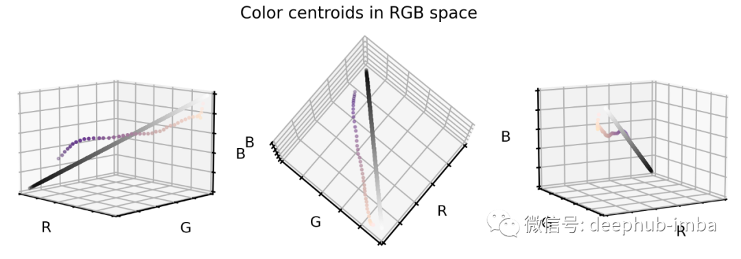
对于原始数据集中的每个颜色值,我们计算到最近的云质心的距离向量。 然后将此距离向量添加到灰度对角线(即重新对齐质心)。 拉伸和剪切颜色值,以确保 99.9% 的所有值都在所需的颜色范围内。
# Create grayscale diagonal centroids (equal numbers to cloud centroids)steps = np.linspace(0.2, 0.8, len(new_centers))# Realign and stretch imagesX_tr_stretch = np.array([x - new_centers[np.argmin(np.linalg.norm(x - new_centers, axis=1))]+ steps[np.argmin(np.linalg.norm(x - new_centers, axis=1))]for x in tqdm(X_tr.reshape(-1, 3))])X_va_stretch = np.array([x - new_centers[np.argmin(np.linalg.norm(x - new_centers, axis=1))]+ steps[np.argmin(np.linalg.norm(x - new_centers, axis=1))]for x in tqdm(X_va.reshape(-1, 3))])X_te_stretch = np.array([x - new_centers[np.argmin(np.linalg.norm(x - new_centers, axis=1))]+ steps[np.argmin(np.linalg.norm(x - new_centers, axis=1))]for x in tqdm(X_te.reshape(-1, 3))])# Stretch and clip dataxmin_tr = np.percentile(X_tr_stretch, 0.05, axis=0)X_tr_stretch -= xmin_trX_va_stretch -= xmin_trX_te_stretch -= xmin_trxmax_tr = np.percentile(X_tr_stretch, 99.95, axis=0)X_tr_stretch /= xmax_trX_va_stretch /= xmax_trX_te_stretch /= xmax_trX_tr_stretch = np.clip(X_tr_stretch, 0, 1)X_va_stretch = np.clip(X_va_stretch, 0, 1)X_te_stretch = np.clip(X_te_stretch, 0, 1)
# Plot color values in 3D spacefig = plt.figure(figsize=(16, 5))stretch_colors = X_tr_stretch[::100]# Loop through 3 different viewsfor i, view in enumerate([[-45, 10], [40, 80], [60, 10]]):ax = fig.add_subplot(1, 3, i + 1, projection="3d")ax.scatter(stretch_colors[:, 0],stretch_colors[:, 1],stretch_colors[:, 2],facecolors=stretch_colors,s=2)ax.set_xlabel("R")ax.set_ylabel("G")ax.set_zlabel("B")ax.xaxis.set_ticklabels([])ax.yaxis.set_ticklabels([])ax.zaxis.set_ticklabels([])ax.view_init(azim=view[0], elev=view[1], vertical_axis="z")ax.set_xlim(0, 1)ax.set_ylim(0, 1)ax.set_zlim(0, 1)plt.suptitle("Colors in realigned and stretched space", fontsize=20)plt.show()
# Convert data back into image spaceX_tr_stretch = X_tr_stretch.reshape(X_tr.shape)X_va_stretch = X_va_stretch.reshape(X_va.shape)X_te_stretch = X_te_stretch.reshape(X_te.shape)# Plot datasetplot_dataset(X_tr_stretch)
# Train PCA decomposition on original RGB valuesfrom sklearn.decomposition import PCApca = PCA()pca.fit(X_tr.reshape(-1, 3))# Transform all data sets into new PCA spaceX_tr_pca = pca.transform(X_tr.reshape(-1, 3))X_va_pca = pca.transform(X_va.reshape(-1, 3))X_te_pca = pca.transform(X_te.reshape(-1, 3))# Stretch and clip dataxmin_tr = np.percentile(X_tr_pca, 0.05, axis=0)X_tr_pca -= xmin_trX_va_pca -= xmin_trX_te_pca -= xmin_trxmax_tr = np.percentile(X_tr_pca, 99.95, axis=0)X_tr_pca /= xmax_trX_va_pca /= xmax_trX_te_pca /= xmax_trX_tr_pca = np.clip(X_tr_pca, 0, 1)X_va_pca = np.clip(X_va_pca, 0, 1)X_te_pca = np.clip(X_te_pca, 0, 1)# Flip first componentX_tr_pca[:, 0] = 1 - X_tr_pca[:, 0]X_va_pca[:, 0] = 1 - X_va_pca[:, 0]X_te_pca[:, 0] = 1 - X_te_pca[:, 0]# Extract a few RGB color valuesX_colors = X_tr_pca[::100].reshape(-1, 3)# Plot color values in 3D spacefig = plt.figure(figsize=(16, 5))# Loop through 3 different viewsfor i, view in enumerate([[-45, 10], [40, 80], [60, 10]]):ax = fig.add_subplot(1, 3, i + 1, projection="3d")ax.scatter(X_colors[:, 0], X_colors[:, 1], X_colors[:, 2], facecolors=X_colors, s=2)ax.set_xlabel("PC1")ax.set_ylabel("PC2")ax.set_zlabel("PC3")ax.xaxis.set_ticklabels([])ax.yaxis.set_ticklabels([])ax.zaxis.set_ticklabels([])ax.view_init(azim=view[0], elev=view[1], vertical_axis="z")ax.set_xlim(0, 1)ax.set_ylim(0, 1)ax.set_zlim(0, 1)plt.suptitle("Colors in PCA space", fontsize=20)plt.show()
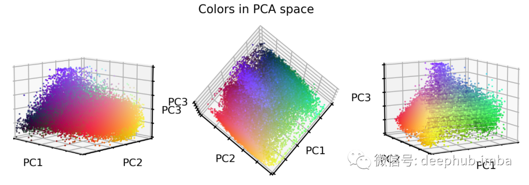
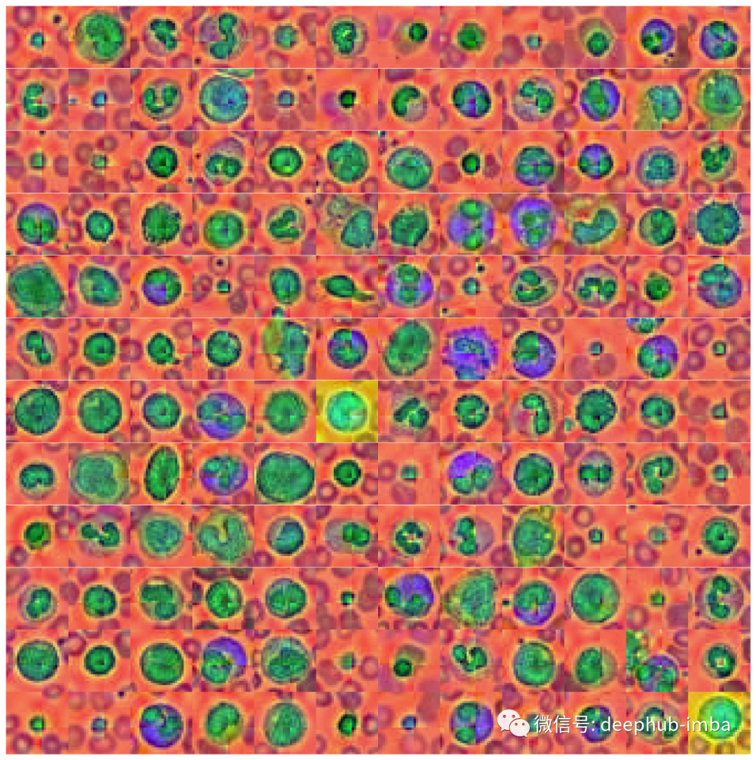
# Convert data back into image spaceX_tr_pca = X_tr_pca.reshape(X_tr.shape)X_va_pca = X_va_pca.reshape(X_va.shape)X_te_pca = X_te_pca.reshape(X_te.shape)# Plot datasetplot_dataset(X_tr_pca)
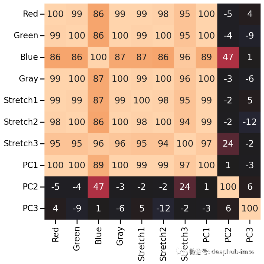
特征的相关性
# Combine all images in one big dataframeX_tr_all = np.vstack([X_tr.T, X_tr_gray.T, X_tr_stretch.T, X_tr_pca.T]).TX_va_all = np.vstack([X_va.T, X_va_gray.T, X_va_stretch.T, X_va_pca.T]).TX_te_all = np.vstack([X_te.T, X_te_gray.T, X_te_stretch.T, X_te_pca.T]).T# Compute correlation matrix between all color featurescorr_all = np.corrcoef(X_tr_all.reshape(-1, X_tr_all.shape[-1]).T)cols = ["Red", "Green", "Blue", "Gray","Stretch1", "Stretch2", "Stretch3","PC1", "PC2", "PC3"]plt.figure(figsize=(8, 8))sns.heatmap(100 * corr_all,square=True,center=0,annot=True,fmt=".0f",cbar=False,xticklabels=cols,yticklabels=cols,)
测试图像分类
# The code for this ResNet architecture was adapted from here:# https://towardsdatascience.com/building-a-resnet-in-keras-e8f1322a49bafrom tensorflow import Tensorfrom tensorflow.keras.layers import (Input, Conv2D, ReLU, BatchNormalization, Add,AveragePooling2D, Flatten, Dense, Dropout)from tensorflow.keras.models import Modeldef relu_bn(inputs: Tensor) -> Tensor:relu = ReLU()(inputs)bn = BatchNormalization()(relu)return bndef residual_block(x: Tensor, downsample: bool, filters: int, kernel_size: int = 3) -> Tensor:y = Conv2D(kernel_size=kernel_size,strides=(1 if not downsample else 2),filters=filters,padding="same")(x)y = relu_bn(y)y = Conv2D(kernel_size=kernel_size, strides=1, filters=filters, padding="same")(y)if downsample:x = Conv2D(kernel_size=1, strides=2, filters=filters, padding="same")(x)out = Add()([x, y])out = relu_bn(out)return outdef create_res_net(in_shape=(28, 28, 3)):inputs = Input(shape=in_shape)num_filters = 32t = BatchNormalization()(inputs)t = Conv2D(kernel_size=3, strides=1, filters=num_filters, padding="same")(t)t = relu_bn(t)num_blocks_list = [2, 2]for i in range(len(num_blocks_list)):num_blocks = num_blocks_list[i]for j in range(num_blocks):t = residual_block(t, downsample=(j == 0 and i != 0), filters=num_filters)num_filters *= 2t = AveragePooling2D(4)(t)t = Flatten()(t)t = Dense(128, activation="relu")(t)t = Dropout(0.5)(t)outputs = Dense(8, activation="softmax")(t)model = Model(inputs, outputs)model.compile(optimizer="adam", loss="sparse_categorical_crossentropy", metrics=["accuracy"])return modeldef run_resnet(X_tr, y_tr, X_va, y_va, epochs=200, verbose=0):"""Support function to train ResNet model"""# Create Modelmodel = create_res_net(in_shape=X_tr.shape[1:])# Creates 'EarlyStopping' callbackfrom tensorflow import kerasearlystopping_cb = keras.callbacks.EarlyStopping(patience=10, restore_best_weights=True)# Train modelhistory = model.fit(X_tr,y_tr,batch_size=120,epochs=epochs,validation_data=(X_va, y_va),callbacks=[earlystopping_cb],verbose=verbose)return model, historydef plot_history(history):"""Support function to plot model history"""# Plots neural network performance metrics for train and validationfig, axs = plt.subplots(1, 2, figsize=(15, 4))results = pd.DataFrame(history.history)results[["accuracy", "val_accuracy"]].plot(ax=axs[0])results[["loss", "val_loss"]].plot(ax=axs[1], logy=True)plt.tight_layout()plt.show()def plot_classification_report(X_te, y_te, model):"""Support function to plot classification report"""# Show classification reportfrom sklearn.metrics import classification_reporty_pred = model.predict(X_te).argmax(axis=1)print(classification_report(y_te.ravel(), y_pred))# Show confusion matrixfrom sklearn.metrics import ConfusionMatrixDisplayfig, ax = plt.subplots(1, 2, figsize=(16, 7))ConfusionMatrixDisplay.from_predictions(y_te.ravel(), y_pred, ax=ax[0], colorbar=False, cmap="inferno_r")from sklearn.metrics import ConfusionMatrixDisplayConfusionMatrixDisplay.from_predictions(y_te.ravel(), y_pred, normalize="true", ax=ax[1],values_format=".1f", colorbar=False, cmap="inferno_r")
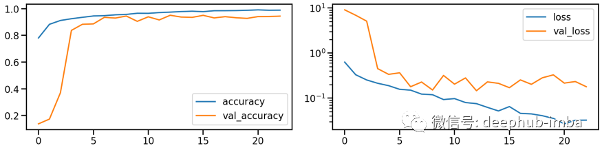
# Train modelmodel_orig, history_orig = run_resnet(X_tr, y_tr, X_va, y_va)# Show model performance during trainingplot_history(history_orig)
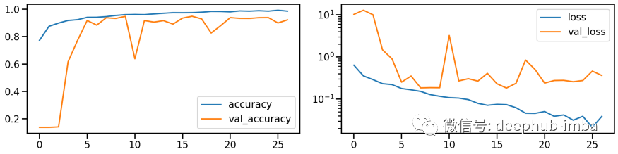
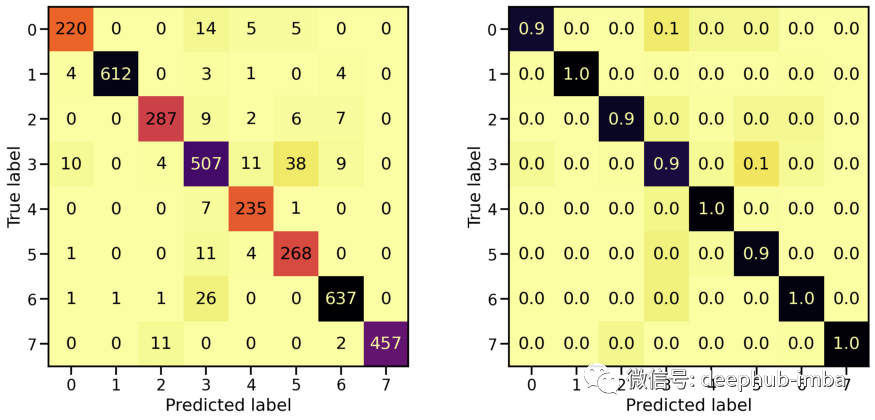
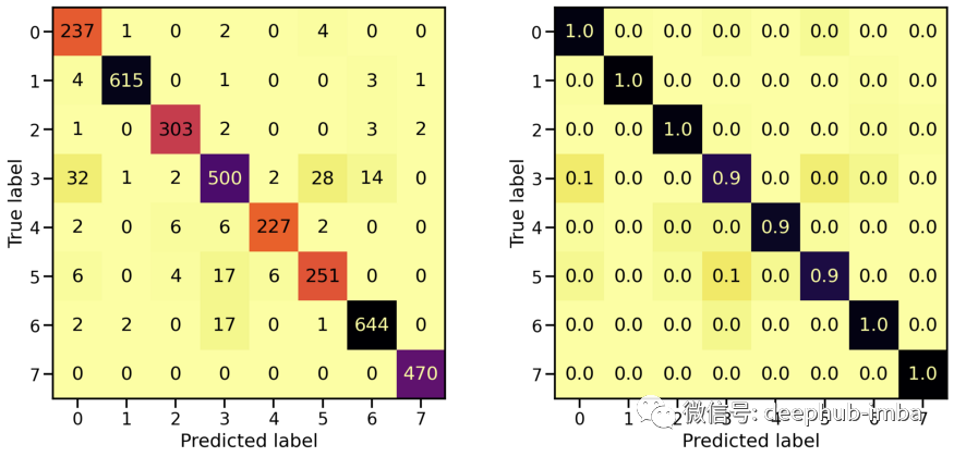
# Evaluate Modelloss_orig_tr, acc_orig_tr = model_orig.evaluate(X_tr, y_tr)loss_orig_va, acc_orig_va = model_orig.evaluate(X_va, y_va)loss_orig_te, acc_orig_te = model_orig.evaluate(X_te, y_te)# Report classification report and confusion matrixplot_classification_report(X_te, y_te, model_orig)Train score: loss = 0.0537 - accuracy = 0.9817Valid score: loss = 0.1816 - accuracy = 0.9492Test score: loss = 0.1952 - accuracy = 0.9421
# Train modelmodel_gray, history_gray = run_resnet(X_tr_gray, y_tr, X_va_gray, y_va)# Show model performance during trainingplot_history(history_gray)
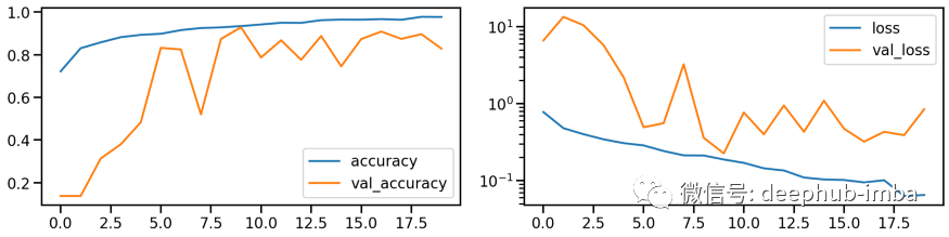
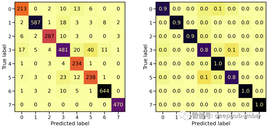
# Evaluate Modelloss_gray_tr, acc_gray_tr = model_gray.evaluate(X_tr_gray, y_tr)loss_gray_va, acc_gray_va = model_gray.evaluate(X_va_gray, y_va)loss_gray_te, acc_gray_te = model_gray.evaluate(X_te_gray, y_te)# Report classification report and confusion matrixplot_classification_report(X_te_gray, y_te, model_gray)Train score: loss = 0.1118 - accuracy = 0.9619Valid score: loss = 0.2255 - accuracy = 0.9287Test score: loss = 0.2407 - accuracy = 0.9220
# Train modelmodel_stretch, history_stretch = run_resnet(X_tr_stretch, y_tr, X_va_stretch, y_va)# Show model performance during trainingplot_history(history_stretch)

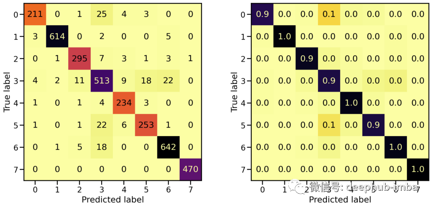
# Evaluate Modelloss_stretch_tr, acc_stretch_tr = model_stretch.evaluate(X_tr_stretch, y_tr)loss_stretch_va, acc_stretch_va = model_stretch.evaluate(X_va_stretch, y_va)loss_stretch_te, acc_stretch_te = model_stretch.evaluate(X_te_stretch, y_te)# Report classification report and confusion matrixplot_classification_report(X_te_stretch, y_te, model_stretch)Train score: loss = 0.0229 - accuracy = 0.9921Valid score: loss = 0.1672 - accuracy = 0.9533Test score: loss = 0.1975 - accuracy = 0.9491
PCA 转换的数据集的分类性能
# Train model
model_pca, history_pca = run_resnet(X_tr_pca, y_tr, X_va_pca, y_va)

# Show model performance during training
plot_history(history_pca)
混淆矩阵
# Evaluate Model
loss_pca_tr, acc_pca_tr = model_pca.evaluate(X_tr_pca, y_tr)
loss_pca_va, acc_pca_va = model_pca.evaluate(X_va_pca, y_va)
loss_pca_te, acc_pca_te = model_pca.evaluate(X_te_pca, y_te)

# Report classification report and confusion matrix
plot_classification_report(X_te_pca, y_te, model_pca)

Train score: loss = 0.0289 - accuracy = 0.9918
Valid score: loss = 0.1459 - accuracy = 0.9509
Test score: loss = 0.1898 - accuracy = 0.9448
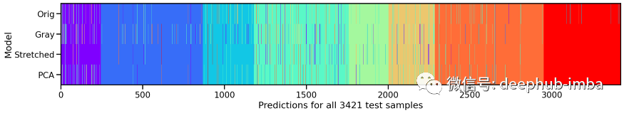
模型对比
# Compute model specific predictionsy_pred_orig = model_orig.predict(X_te).argmax(axis=1)y_pred_gray = model_gray.predict(X_te_gray).argmax(axis=1)y_pred_stretch = model_stretch.predict(X_te_stretch).argmax(axis=1)y_pred_pca = model_pca.predict(X_te_pca).argmax(axis=1)# Aggregate all model predictionstarget = y_te.ravel()predictions = np.array([y_pred_orig, y_pred_gray, y_pred_stretch, y_pred_pca])[:, np.argsort(target)]# Plot model individual predictionsplt.figure(figsize=(20, 3))plt.imshow(predictions, aspect="auto", interpolation="nearest", cmap="rainbow")plt.xlabel(f"Predictions for all {predictions.shape[1]} test samples")plt.ylabel("Model")plt.yticks(ticks=range(4), labels=["Orig", "Gray", "Stretched", "PCA"]);
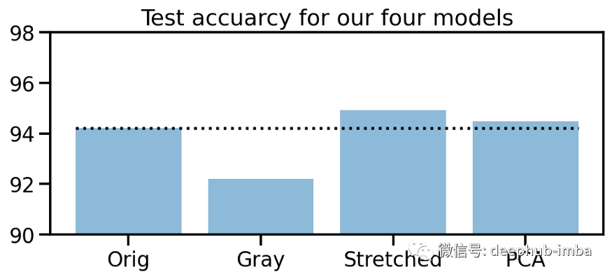
# Collect accuraciesaccs_te = np.array([acc_orig_te, acc_gray_te, acc_stretch_te, acc_pca_te]) * 100# Plot accuraciesplt.figure(figsize=(8, 3))plt.title("Test accuracy for our four models")plt.bar(["Orig", "Gray", "Stretched", "PCA"], accs_te, alpha=0.5)plt.hlines(accs_te[0], -0.4, 3.4, colors="black", linestyles="dotted")plt.ylim(90, 98);
模型叠加
# Compute prediction probabilities for all models and data setsy_prob_tr_orig = model_orig.predict(X_tr)y_prob_tr_gray = model_gray.predict(X_tr_gray)y_prob_tr_stretch = model_stretch.predict(X_tr_stretch)y_prob_tr_pca = model_pca.predict(X_tr_pca)y_prob_va_orig = model_orig.predict(X_va)y_prob_va_gray = model_gray.predict(X_va_gray)y_prob_va_stretch = model_stretch.predict(X_va_stretch)y_prob_va_pca = model_pca.predict(X_va_pca)y_prob_te_orig = model_orig.predict(X_te)y_prob_te_gray = model_gray.predict(X_te_gray)y_prob_te_stretch = model_stretch.predict(X_te_stretch)y_prob_te_pca = model_pca.predict(X_te_pca)# Combine prediction probabilities into meta data setsy_prob_tr = np.concatenate([y_prob_tr_orig, y_prob_tr_gray, y_prob_tr_stretch, y_prob_tr_pca], axis=1)y_prob_va = np.concatenate([y_prob_va_orig, y_prob_va_gray, y_prob_va_stretch, y_prob_va_pca], axis=1)y_prob_te = np.concatenate([y_prob_te_orig, y_prob_te_gray, y_prob_te_stretch, y_prob_te_pca], axis=1)# Combine training and validation datasety_prob_train = np.concatenate([y_prob_tr, y_prob_va], axis=0)y_train = np.concatenate([y_tr, y_va], axis=0).ravel()
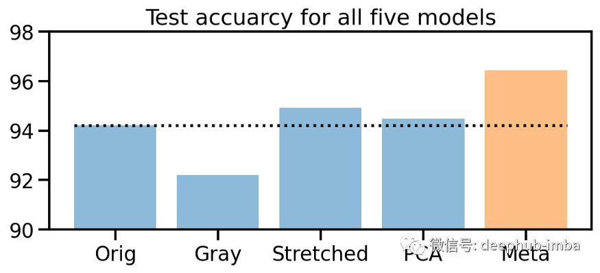
from sklearn.neural_network import MLPClassifier# Create MLP classifierclf = MLPClassifier(hidden_layer_sizes=(32, 16), activation="relu", solver="adam", alpha=0.42, batch_size=120,learning_rate="adaptive", learning_rate_init=0.001, max_iter=100, shuffle=True, random_state=24,early_stopping=True, validation_fraction=0.15)# Train modelclf.fit(y_prob_train, y_train)# Compute prediction accuracy of meta classifieracc_meta_te = np.mean(clf.predict(y_prob_te) == y_te.ravel())# Collect accuraciesaccs_te = np.array([acc_orig_te, acc_gray_te, acc_stretch_te, acc_pca_te, 0]) * 100accs_meta = np.array([0, 0, 0, 0, acc_meta_te]) * 100# Plot accuraciesplt.figure(figsize=(8, 3))plt.title("Test accuracy for all five models")plt.bar(["Orig", "Gray", "Stretched", "PCA", "Meta"], accs_te, alpha=0.5)plt.bar(["Orig", "Gray", "Stretched", "PCA", "Meta"], accs_meta, alpha=0.5)plt.hlines(accs_te[0], -0.4, 4.4, colors="black", linestyles="dotted")plt.ylim(90, 98);
本文地址:
https://miykael.github.io/blog/2021/color_engineering_medmnist/
作者:michael notter
评论