
图像配准:基于 OpenCV 的高效实现
点击下方卡片,关注“新机器视觉”公众号
重磅干货,第一时间送达
在这篇文章中,我将对图像配准进行一个简单概述,展示一个最小的 OpenCV 实现,并展示一个可以使配准过程更加高效的简单技巧。
什么是图像配准
图像配准被定义为将不同成像设备或传感器在不同时间和角度拍摄的两幅或多幅图像,或来自同一场景的两幅或多幅图像叠加起来,以几何方式对齐图像以进行分析的过程(Zitová 和 Flusser,2003 年)。
百度百科给出的解释
图像配准:图像配准(Image registration)就是将不同时间、不同传感器(成像设备)或不同条件下(天候、照度、摄像位置和角度等)获取的两幅或多幅图像进行匹配、叠加的过程,它已经被广泛地应用于遥感数据分析、计算机视觉、图像处理等领域。
医学科学、遥感和计算机视觉都使用图像配准。
有两种主要方法:
经典计算机视觉方法(使用 OpenCV)——我们将在本文中关注的内容
基于深度学习的方法
虽然后者可以更好地工作,但它可能需要一些“域”适应(在你的数据上微调神经网络)并且可能计算量太大。
使用 OpenCV 进行图像配准
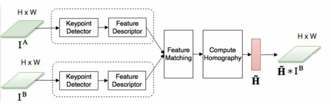
基于特征的方法:由单应变换关联的图像对
此操作试图发现两张照片之间的匹配区域并在空间上对齐它们以最大限度地减少错误。
我们的目标是找到一个单应性矩阵 H,它告诉我们需要如何修改其中一张图像,使其与另一张图像完美对齐。
第 1 步:关键点检测
关键点定义了图像中一个独特的小区域(角、边缘、图案)。关键点检测器的一个重要方面是找到的区域应该对图像变换(例如定位、比例和亮度)具有鲁棒性,因为这些区域很可能出现在我们试图对齐的两个图像中。有许多执行关键点检测的算法,例如 SIFT、ORB、AKAZE、SURF 等。
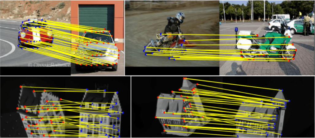
第 2 步:特征匹配
现在我们必须匹配来自两个图像的关键点,这些关键点实际上对应于同一点。
第 3 步:单应性
单应性通常由一个 3x3 矩阵表示,它描述了应该应用于一个图像以与另一个图像对齐的几何变换。
第 4 步:图像变形
找到单应性矩阵后,我们可以用它来对齐图像。下面是该过程的代码:
import numpy as npimport cv2 as cvimport matplotlib.pyplot as pltimg1 = cv.imread('image1.jpg', cv.IMREAD_GRAYSCALE) # referenceImageimg2 = cv.imread('image2.jpg', cv.IMREAD_GRAYSCALE) # sensedImage# Initiate SIFT detectorsift_detector = cv.SIFT_create()# Find the keypoints and descriptors with SIFTkp1, des1 = sift_detector.detectAndCompute(img1, None)kp2, des2 = sift_detector.detectAndCompute(img2, None)# BFMatcher with default paramsbf = cv.BFMatcher()matches = bf.knnMatch(des1, des2, k=2)# Filter out poor matchesgood_matches = []for m,n in matches:if m.distance < 0.75*n.distance:good_matches.append(m)matches = good_matchespoints1 = np.zeros((len(matches), 2), dtype=np.float32)points2 = np.zeros((len(matches), 2), dtype=np.float32)for i, match in enumerate(matches):points1[i, :] = kp1[match.queryIdx].ptpoints2[i, :] = kp2[match.trainIdx].pt# Find homographyH, mask = cv2.findHomography(points1, points2, cv2.RANSAC)# Warp image 1 to align with image 2img1Reg = cv2.warpPerspective(img1, H, (img2.shape[1], img2.shape[0]))cv.imwrite('aligned_img1.jpg', img1Reg)The problem is that this matrix H is found via a compute-intensive optimization process.
高效的图像配准
无论您为每个步骤选择的参数如何,对执行时间影响最大的是图像的分辨率。您可以大幅调整它们的大小,但如果您需要对齐的图像具有原始分辨率,会发生什么情况?
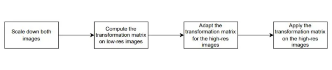
幸运的是,有办法解决这个问题。事实证明,您可以计算低分辨率图像的变换,然后调整此变换以适用于全分辨率图像。
详细步骤:
调整图像大小
在低分辨率图像上计算矩阵 H
变换矩阵 H 使其适用于全分辨率图像
将新矩阵应用于原始图像。
第 3 步可能是这里最不明显的部分,所以让我们看看它是如何工作的:
我们想要调整在低分辨率图像上计算的变换以适用于高分辨率图像。因此,我们希望高分辨率图像中的每个像素执行以下操作:
缩小到低分辨率 -> 应用变换 H -> 放大到高分辨率
幸运的是,所有这些步骤都只是矩阵乘法,我们可以将所有这些步骤组合在一个单一的转换中。
设 H 为您计算出的变换。您可以将 H 乘以另一个单应性 A,得到 AH = H',其中 H' 是进行两种变换的单应性,相当于先应用 H,然后应用 A。
下面是详细代码:
import numpy as npimport cv2 as cvimport matplotlib.pyplot as pltimg1 = cv.imread('image1.jpg', cv.IMREAD_GRAYSCALE) # referenceImageimg2 = cv.imread('image2.jpg', cv.IMREAD_GRAYSCALE) # sensedImage# Resize the image by a factor of 8 on each side. If your images are# very high-resolution, you can try to resize even more, but if they are# already small you should set this to something less agressive.resize_factor = 1.0/8.0img1_rs = cv.resize(img1, (0,0), fx=resize_factor, fy=resize_factor)img2_rs = cv.resize(img2, (0,0), fx=resize_factor, fy=resize_factor)# Initiate SIFT detectorsift_detector = cv.SIFT_create()# Find the keypoints and descriptors with SIFT on the lower resolution imageskp1, des1 = sift_detector.detectAndCompute(img1_rs, None)kp2, des2 = sift_detector.detectAndCompute(img2_rs, None)# BFMatcher with default paramsbf = cv.BFMatcher()matches = bf.knnMatch(des1, des2, k=2)# Filter out poor matchesgood_matches = []for m,n in matches:if m.distance < 0.75*n.distance:good_matches.append(m)matches = good_matchespoints1 = np.zeros((len(matches), 2), dtype=np.float32)points2 = np.zeros((len(matches), 2), dtype=np.float32)for i, match in enumerate(matches):points1[i, :] = kp1[match.queryIdx].ptpoints2[i, :] = kp2[match.trainIdx].pt# Find homographyH, mask = cv2.findHomography(points1, points2, cv2.RANSAC)# Get low-res and high-res sizeslow_height, low_width = img1_rs.shapeheight, width = img1.shapelow_size = np.float32([[0, 0], [0, low_height], [low_width, low_height], [low_width, 0]])high_size = np.float32([[0, 0], [0, height], [width, height], [width, 0]])# Compute scaling transformationsscale_up = cv.getPerspectiveTransform(low_size, high_size)scale_down = cv.getPerspectiveTransform(high_size, low_size)# Combine the transformations. Remember that the order of the transformation# is reversed when doing matrix multiplication# so this is actualy scale_down -> H -> scale_uph_and_scale_up = np.matmul(scale_up, H)scale_down_h_scale_up = np.matmul(h_and_scale_up, scale_down)# Warp image 1 to align with image 2img1Reg = cv2.warpPerspective(img1,scale_down_h_scale_up,(img2.shape[1], img2.shape[0]))cv.imwrite('aligned_img1.jpg', img1Reg)
本文仅做学术分享,如有侵权,请联系删文。