
Python 做机器学习得先学它吧
想啥呢,难道不是 NumPy 吗?

如果还没学,看这个包会。
如果早会了,拉到最后,有深入篇等你哦。
上一篇中,对 NumPy 中最基本的概念 ndarray 对象对了介绍,图文并茂,让大家可以快速掌握它的基本要素、内部结构以及索引和切片等必备知识。
本篇进一步把以下针对数组的常用操作精简浓缩,
创建 约简 排序 堆垒 拼接 展平
import numpy as np
1数组创建
创建全是 1的数组,注意参数是表示数组shape的元组。
arr_ones = np.ones((3,4))
arr_ones
array([[1., 1., 1., 1.],
       [1., 1., 1., 1.],
       [1., 1., 1., 1.]])
arr_ones.dtype
dtype('float64')
创建全是 0的数组
arr_zeros = np.zeros((3,4))
arr_zeros
array([[0., 0., 0., 0.],
       [0., 0., 0., 0.],
       [0., 0., 0., 0.]])
创建单位矩阵
# 返回一个二维数组,对角线上元素全是 1,其他元素全为 0。
arr_eye = np.eye(3, dtype=np.int64)
arr_eye
array([[1, 0, 0],
       [0, 1, 0],
       [0, 0, 1]])
创建给定 shape和dtype的新数组,而无需初始化元素。
arr_empty = np.empty((3,4))
arr_empty
array([[0., 0., 0., 0.],
       [0., 0., 0., 0.],
       [0., 0., 0., 0.]])
创建一个具有给定 shape和dtype的新数组,并以fill_value的值填充元素。
# np.full(shape, fill_value, dtype=None, order='C')
arr_full = np.full((3, 3), 3.1415)
arr_full
array([[3.1415, 3.1415, 3.1415],
       [3.1415, 3.1415, 3.1415],
       [3.1415, 3.1415, 3.1415]])
创建一个数组,元素为给定间隔的均匀分布的值(不包括 stop)。
# arange([start,] stop[, step,], dtype=None)

np.arange(10)
array([0, 1, 2, 3, 4, 5, 6, 7, 8, 9])
# 起,止(不包括),步长
np.arange(3, 10, 2)
array([3, 5, 7, 9])
返回在区间 [ start,stop] 中计算出的num个均匀间隔的数值,包括stop。
# np.linspace(start, stop, num=50, ...)

np.linspace(0, 10, num=5)
2数组约简
常用统计函数
如 sum,mean,std,var,min,max 等函数。
data = np.arange(18).reshape(2, 3, 3)
data
array([[[ 0,  1,  2],
        [ 3,  4,  5],
        [ 6,  7,  8]],

       [[ 9, 10, 11],
        [12, 13, 14],
        [15, 16, 17]]])
# 没有指定 `axis` 参数,说明对所有轴约简
data.sum()
153
A.sum()对应的数学公式为
np.sum(data, axis=0)
array([[ 9, 11, 13],
       [15, 17, 19],
       [21, 23, 25]])
A.sum(axis=0)对应的数学公式为
np.sum(data, axis=1)
array([[ 9, 12, 15],
       [36, 39, 42]])
A.sum(axis=1)对应的数学公式为
np.sum(data, axis=(0,1))
array([45, 51, 57])
A.sum(axis=(0,1))对应的数学公式为
# 沿轴取最小值
data.min(axis=1)
array([[ 0,  1,  2],
       [ 9, 10, 11]])
# 标准差
data.std(axis=0) # 或者 a = np.std(data)
array([[4.5, 4.5, 4.5],
       [4.5, 4.5, 4.5],
       [4.5, 4.5, 4.5]])
a = np.std(data)
a*a
26.916666666666664
#方差
data.var()
26.916666666666668
# 也可以按轴计算标准差
data.std(axis=1)
array([[2.44948974, 2.44948974, 2.44948974],
       [2.44948974, 2.44948974, 2.44948974]])
约简操作
NumPy 中对数组的约简操作是沿着某个或某些轴按某种运算减少数组中元素数量的操作。
例如丢弃某个维度,将数据沿这个维度压缩为单个单元,从而批量减少数据量。如上文中统计数据的函数,实质是约简操作。
另外,还有如下这些常用函数,
argmax: 返回 array 中数值最大数的下标,默认将输入 array 视作一维,出现相同的最大,返回第一次出现的。 argmin: 返回 array 中数值最小数的下标,默认将输入 array 视作一维,出现相同的最小,返回第一次出现的。 reduce 和 accumulate。
当我们处理一维数组时,是通过下标对所有元素进行加法、减法、最大/最小值、求和、平均值、标准差等。
data = np.array(np.arange(16))
data
array([ 0, 1, 2, 3, 4, 5, 6, 7, 8, 9, 10, 11, 12, 13, 14, 15])
data.mean()
7.5
当处理更高维度数组时,可以看到 numpy 可以沿任何给定的轴进行约简求和。例如,考虑一个二维数组/矩阵。
# 没有指定轴,指所有元素
data_2d = data.reshape((4,4))
data_2d.mean()
7.5
例子,统计学生三门课的成绩。
# 假设每一行对应一个学生的三门课的成绩,共十个学生
np.random.seed(1)
data_2d = np.random.randint(60,100,(10,3))
data_2d
array([[97, 72, 68],
       [69, 71, 65],
       [75, 60, 76],
       [61, 72, 67],
       [66, 85, 80],
       [97, 78, 80],
       [71, 88, 89],
       [74, 64, 83],
       [83, 90, 92],
       [82, 73, 69]])
# 统计每门课的平均成绩
data_2d.mean(axis = 1)
array([79.        , 68.33333333, 70.33333333, 66.66666667, 77.        ,
       85.        , 82.66666667, 73.66666667, 88.33333333, 74.66666667])
# 分别计算每个学生三门课的总成绩和平均成绩
data_2d.sum(axis = 1), data_2d.mean(axis = 1)
(array([237, 205, 211, 200, 231, 255, 248, 221, 265, 224]),
 array([79.        , 68.33333333, 70.33333333, 66.66666667, 77.        ,
        85.        , 82.66666667, 73.66666667, 88.33333333, 74.66666667]))
找出每门课的最高成绩的学生
data_2d.argmax(axis=0)
array([1, 6, 4])
找出每个学生成绩最高的那门课
ind = data_2d.argmax(axis=1)
ind
array([1, 0, 1, 1, 2, 0, 1, 0, 0, 2])
# 使用花式索引挑出每个学生成绩最好那门课的成绩
data_2d[np.arange(10), ind]
array([63, 99, 96, 84, 98, 99, 97, 73, 80, 78])
# 而如果这样来引用,就得到了完全不同的结果,想想这是在干吗?
data_2d[:, ind]
array([[63, 60, 63, 63, 63, 60, 63, 60, 60, 63],
       [69, 99, 69, 69, 79, 99, 69, 99, 99, 79],
       [96, 81, 96, 96, 83, 81, 96, 81, 81, 83],
       [84, 66, 84, 84, 84, 66, 84, 66, 66, 84],
       [61, 72, 61, 61, 98, 72, 61, 72, 72, 98],
       [83, 99, 83, 83, 84, 99, 83, 99, 99, 84],
       [97, 77, 97, 97, 85, 77, 97, 77, 77, 85],
       [68, 73, 68, 68, 69, 73, 68, 73, 73, 69],
       [76, 80, 76, 76, 65, 80, 76, 80, 80, 65],
       [60, 75, 60, 60, 78, 75, 60, 75, 75, 78]])
约简但仍然保持维数,不丢失轴。
# a.mean(axis=None, dtype=None, out=None, keepdims=False)
data_2d.mean(axis=1, keepdims=True)
array([[62.        ],
       [82.33333333],
       [86.66666667],
       [78.        ],
       [77.        ],
       [88.66666667],
       [86.33333333],
       [70.        ],
       [73.66666667],
       [71.        ]])
reduce 方法
reduce 方法沿着 axis 轴对 array 进行操作,可以实现沿着 axis 轴的所有子数组或者元素进行相关运算。
np.add.reduce(data_2d)
array([782, 757, 788])
累积约简
accumulate 方法
accumulate 方法和 reduce 方法类似,但是它返回的数组和输入数组的 shape 相同,即保留了中间计算结果。
np.add.accumulate(data_2d)
array([[ 60,  63,  63],
       [159, 132, 142],
       [240, 228, 225],
       [306, 312, 309],
       [378, 373, 407],
       [477, 456, 491],
       [554, 553, 576],
       [627, 621, 645],
       [707, 697, 710],
       [782, 757, 788]])
numpy.cumsum 方法
numpy.cumsum(a, axis=None, dtype=None, out=None)
axis=0,按照行累加。
axis=1,按照列累加。
axis 不给定具体值,就把 numpy 数组当成一个一维数组。
沿给定轴的元素的累加和。
a = np.array([[1,2,3], [4,5,6]])
a
array([[1, 2, 3],
       [4, 5, 6]])
np.cumsum(a, axis = 0)
array([[1, 2, 3],
       [5, 7, 9]])
np.cumsum(a, axis = 1)
array([[ 1,  3,  6],
       [ 4,  9, 15]])
np.cumsum(a)
array([ 1, 3, 6, 10, 15, 21])
# 指定输出的数据类型
np.cumsum(a, dtype=float)
array([ 1., 3., 6., 10., 15., 21.])
np.cumsum(a, axis=0)
array([[1, 2, 3],
       [5, 7, 9]])
np.cumsum(a, axis=1)
array([[ 1,  3,  6],
       [ 4,  9, 15]])
3数组排序
先准备工作,创建数组并打乱顺序。
data = np.array(np.arange(12))
id(data), data
(140464554206752, array([ 0, 1, 2, 3, 4, 5, 6, 7, 8, 9, 10, 11]))
# 打乱顺序
np.random.shuffle(data)
id(data), data
(140464554206752, array([ 4, 2, 7, 9, 0, 6, 10, 5, 11, 1, 8, 3]))
data = data.reshape(3, 4)
data
array([[ 4,  2,  7,  9],
       [ 0,  6, 10,  5],
       [11,  1,  8,  3]])
对数组元素按轴排序
np.sort(a, axis=-1, kind='quicksort', order=None),默认是按最后一个轴排序的
A1 = np.sort(data_2d)
A2 = np.sort(data_2d, axis=-1)
print(A1)
print(A2)
[[68 72 97]
 [65 69 71]
 [60 75 76]
 [61 67 72]
 [66 80 85]
 [78 80 97]
 [71 88 89]
 [64 74 83]
 [83 90 92]
 [69 73 82]]
[[68 72 97]
 [65 69 71]
 [60 75 76]
 [61 67 72]
 [66 80 85]
 [78 80 97]
 [71 88 89]
 [64 74 83]
 [83 90 92]
 [69 73 82]]
# 也可以选择排序算法
data_0 = np.sort(data, kind='quicksort')
data_0
array([[ 0,  3, 10, 11],
       [ 2,  4,  6,  7],
       [ 1,  5,  8,  9]])
(id(data), id(data_0))
(140608173829056, 140608173889136)
假如需要按某列对所有行进行排序,如何操作?
# 自定义一个结构体,以便按某个成员的值排序
dtype = np.dtype([('student', int), ('point',  int), ('index',  float)])

data = np.array([
    (4551109, 94,   5.55772148),
    (4156490, 134,  5.5090355),
    (4822166, 4069, 9.25039792),
    (4367966, 257,  7.3435601),
    (4426400, 3390, 9.19012117),
    (4367966, 301,  7.32418416),
    (3919410, 2566, 8.92952842),
    (4538580, 138,  6.02654709),
    (4214718, 252,  6.89835322),
    (4426400, 3155, 9.59667276)], dtype=dtype)
data.shape
(10,)
data = np.sort(data, order='point')
[d for d in data]
[(4551109, 94, 5.55772148),
 (4156490, 134, 5.5090355),
 (4538580, 138, 6.02654709),
 (4214718, 252, 6.89835322),
 (4367966, 257, 7.3435601),
 (4367966, 301, 7.32418416),
 (3919410, 2566, 8.92952842),
 (4426400, 3155, 9.59667276),
 (4426400, 3390, 9.19012117),
(4822166, 4069, 9.25039792)]4拼接与堆叠
沿着已有轴拼接用 concatenating,不增加新轴。创建新轴再堆起来构建更高维度的数组用 stack。
使用
np.concatenate沿着已有的轴拼接数组
np.concatenate
data = np.arange(4).reshape(2, 2)

print('axis=0: \n', np.concatenate([data, data], axis=0))
print('axis=1: \n', np.concatenate([data, data], axis=1))
axis=0:
 [[0 1]
 [2 3]
 [0 1]
 [2 3]]
axis=1:
 [[0 1 0 1]
 [2 3 2 3]]
numpy.stack
使用 numpy.stack(arrays, axis=0),沿着新轴拼接数组序列。
numpy.stack(arrays, axis=0)
参数: arrays:序列中每个数组必须具有相同的形状。参数 axis指定新轴在结果尺寸中的索引。例如,axis=0,新增第一个维度,如果axis=-1,则新增最后一个维度。返回:堆叠数组比输入数组多一个轴。
x = np.array([2, 3, 4])
y = np.array([3, 4, 5])
x, y
(array([2, 3, 4]), array([3, 4, 5]))
# 下面代码将 x y 都增加一个轴,shape 都变成 [1,3] [1,3],再沿着新增的 0-轴组合成新的数组。
xy = np.stack((x, y))
xy
array([[2, 3, 4],
       [3, 4, 5]])
xy[0,:]
array([2, 3, 4])
# 下面代码将 x y 都增加一个轴,shape 都变成 [3,1] [3,1],再沿着新增的 1-轴组合成新的数组。
xy = np.stack((x, y), axis=-1)
xy
array([[2, 3],
       [3, 4],
       [4, 5]])
# 下面代码将 xy 增加一个轴,shape 变成 [3,2,1],再沿着新增的 1-轴组合成新的数组。
xy2 = np.stack((xy, xy), axis=-1)
xy2
array([[[2, 2],
        [3, 3]],

       [[3, 3],
        [4, 4]],

       [[4, 4],
        [5, 5]]])
print(xy2[:,:,0])
print('-------')
print(xy2[:,:,1])
[[2 3]
 [3 4]
 [4 5]]
-------
[[2 3]
 [3 4]
 [4 5]]
# 其他例子
x1 = np.arange(9).reshape((3,3))
x2 = np.arange(10,19,1).reshape((3,3))

print(x1)
print('------------')
print(x2)

y2 = np.stack((x1,x2),axis=0)
y2
[[0 1 2]
 [3 4 5]
 [6 7 8]]
------------
[[10 11 12]
 [13 14 15]
 [16 17 18]]


array([[[ 0,  1,  2],
        [ 3,  4,  5],
        [ 6,  7,  8]],

       [[10, 11, 12],
        [13, 14, 15],
        [16, 17, 18]]])
arrays = [np.random.randn(3, 4) for _ in range(10)]
np.stack(arrays, axis=0).shape
(10, 3, 4)
np.stack(arrays, axis=1).shape
(3, 10, 4)
上面的代码相当于,先将 shape: (3, 4) 改成 (3, 1, 4),再沿着中间的轴堆叠,从而将 shape 中间的 1 变成了 10。
np.stack(arrays, axis=2).shape
(3, 4, 10)
data
array([[0, 1],
       [2, 3]])
np.concatenate 用于堆垒
如果想 np.concatenate像np.stack那样增加一个维度,则需要先对数组增加一个轴,然后再使用np.concatenate沿着那个轴拼接。
dd = np.concatenate([data[np.newaxis,...], data[np.newaxis,...]])
dd
array([[[0, 1],
        [2, 3]],

       [[0, 1],
        [2, 3]]])
拆分数组
data = np.array([[[1, 2, 3],[4, 5, 6],[7, 8, 9]],[[-1, -2, -3],[-4, -5, -6],[-7, -8, -9]]])
data
array([[[ 1,  2,  3],
        [ 4,  5,  6],
        [ 7,  8,  9]],

       [[-1, -2, -3],
        [-4, -5, -6],
        [-7, -8, -9]]])
x, y = data[0, ...], data[1, ...]

print(x)
print(y)
[[1 2 3]
 [4 5 6]
 [7 8 9]]
[[-1 -2 -3]
 [-4 -5 -6]
 [-7 -8 -9]]

5数组展平
将数组展平为一维数组, numpy.ravel() vs numpy.flatten()。
data = np.arange(12).reshape((3, 2,2))
data
array([[[ 0,  1],
        [ 2,  3]],

       [[ 4,  5],
        [ 6,  7]],

       [[ 8,  9],
        [10, 11]]])
# 按行展开,即 C 语言风格
data_flatten = data.flatten()
data_flatten
array([ 0, 1, 2, 3, 4, 5, 6, 7, 8, 9, 10, 11])
# 按列展开,即 FORTRAN 语言风格
data_flatten = data.flatten(order="F")
data_flatten
array([ 0, 4, 8, 2, 6, 10, 1, 5, 9, 3, 7, 11])
# 修改 data_flatten 的元素,看是否影响原始数组
data_flatten[0] = 110
data
array([[[ 0,  1],
        [ 2,  3]],

       [[ 4,  5],
        [ 6,  7]],

       [[ 8,  9],
        [10, 11]]])
 # 按行展开,C 语言风格
data_ravel = data.ravel()
data_ravel
array([ 0, 1, 2, 3, 4, 5, 6, 7, 8, 9, 10, 11])
# 修改 data_ravel 的元素,看是否影响原始数组
data_ravel[0] = 110
data
array([[[110,   1],
        [  2,   3]],

       [[  4,   5],
        [  6,   7]],

       [[  8,   9],
        [ 10,  11]]])
# 按行展开 F 风格
data[0] = 0
data_ravel = data.ravel(order='F')
data_ravel
array([ 0, 4, 8, 0, 6, 10, 0, 5, 9, 0, 7, 11])
# 修改 F 风格的 data_ravel 的元素,看是否影响原始数组
data_ravel[0] = 110
data
array([[[ 0,  0],
        [ 0,  0]],

       [[ 4,  5],
        [ 6,  7]],

       [[ 8,  9],
        [10, 11]]])
ravel()和flatten()两者实现的功能是一致的(将多维数组降到一维)两者的区别在于返回拷贝(copy)还是返回视图(view) numpy.flatten()返回一份拷贝,对拷贝所做的修改不会影响原始矩阵而 numpy.ravel()一般情况下返回的是视图(view),修改会影响原始矩阵。但是当数组不是C连续(contiguous)时,numpy.ravel()返回的也会是拷贝。
# 查看是否 C 连续
data.flags
  C_CONTIGUOUS : True
  F_CONTIGUOUS : False
  OWNDATA : False
  WRITEABLE : True
  ALIGNED : True
  WRITEBACKIFCOPY : False
  UPDATEIFCOPY : False
上面例子中的 data 数组如下,
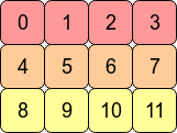

data 数据在内存中是连续的。但是,如果当以 order='F' 展开时,是按 [0,4,8,1,5,9,2,6,10,3,7,11] 这个顺序,它这个顺序从内存地址上看就不是连续了,因此返回的是拷贝。NumPy 快速修炼必备知识 1
NumPy 进阶 之 数组初探 3: 图解 view 和 copy 2