用 Pandas 分析均线交叉策略收益率-技术圈

在这篇文章中，我们会利用上一篇文章中的均线交叉策略回测中获得的结果（《用 Python 基于均线交叉策略进行回测》），并花一些时间更深入地挖掘权益曲线并生成一些关键绩效指标和一些有趣的数据分析。为完整起见，文末扫码加入宽客量化俱乐部可以获得生成策略回测结果所需的所有代码和Jupyter Notebook文件，并绘制了权益曲线图。

#导入相关模块import pandas as pdimport numpy as npfrom pandas_datareader import datafrom math import sqrtimport matplotlib.pyplot as plt

#将数据下载到 DataFrame 并创建移动平均列sp500 = data.DataReader('^GSPC', 'yahoo',start='1/1/2000')sp500['42d'] = np.round(sp500['Close'].rolling(window=42).mean(),2)sp500['252d'] = np.round(sp500['Close'].rolling(window=252).mean(),2)
#创建具有移动平均价差差异的列sp500['42-252'] = sp500['42d'] - sp500['252d']
#将所需的点数设置为点差的阈值并创建包含策略'Stance'的列X = 50sp500['Stance'] = np.where(sp500['42-252'] > X, 1, 0)sp500['Stance'] = np.where(sp500['42-252'] < X, -1, sp500['Stance'])sp500['Stance'].value_counts()
#创建包含每日市场回报和策略每日回报的列sp500['Market Returns'] = np.log(sp500['Close'] / sp500['Close'].shift(1))sp500['Strategy'] = sp500['Market Returns'] * sp500['Stance'].shift(1)
#将策略起始权益设置为 1（即 100%）并生成权益曲线sp500['Strategy Equity'] = sp500['Strategy'].cumsum() + 1
#显示权益曲线图sp500['Strategy Equity'].plot()

我们计划分析如下指标：

a) 滚动 1 年年化波动率

b) 滚动 1 年命中率

c) 滚动 1 年回报

d) 每日收益图表

e) 每日收益分布直方图

第一步是创建一个仅包含我们需要的数据的新 DataFrame，即策略权益曲线以及每日策略收益。可以按如下方式完成的：

strat = pd.DataFrame([sp500['Strategy Equity'], sp500['Strategy']]).transpose()

现在我们必须构建 DataFrame 以包含我们需要计算上面系列所需的所有原始数据，我们希望绘制这些数据。代码如下：

#创建表示每天回报是正数、负数还是持平的列。strat['win'] = (np.where(strat['Strategy'] > 0, 1,0)) strat['loss'] = (np.where(strat['Strategy'] < 0, 1,0)) strat['scratch'] = (np.where(strat['Strategy'] == 0, 1,0)) 
#使用上面创建的每一列的累积总和来创建列 str['wincum'] = (np.where(strat['Strategy'] > 0, 1,0)).cumsum()strat['losscum'] = (np.where(strat['Strategy'] < 0, 1,0)).cumsum() strat['scratchcum'] = (np.where(strat['Strategy'] == 0, 1,0)).cumsum() 
#创建一个包含连续交易日总和的列 - 我们稍后将使用它来创建我们的百分比strat['days'] = (strat['wincum'] + strat['losscum'] + strat['scratchcum']) 
#创建显示赢/输/持平天数的 252 天滚动总和的列strat['rollwin'] = strat['win'].rolling(window=252).sum() strat['rollloss'] = strat['loss'].rolling(window=252).sum() strat['rollscratch'] = strat['scratch'].rolling(window=252).sum() 
#创建具有命中率和损失率数据的列strat['hitratio'] = strat['wincum'] / (strat['wincum']+strat['losscum']) strat['lossratio'] = 1- strat['hitratio'] 
#创建具有滚动 252 天命中率和损失率数据的列strat['rollhitratio'] = strat['hitratio'].rolling(window=252).mean()strat['rolllossratio'] =1 -strat['rollhitratio' ]
#创建具有滚动 12 个月回报的列strat['roll12mret'] = strat['Strategy'].rolling(window=252).sum() 
#创建包含平均赢利、平均损失和平均每日回报数据的列strat['averagewin'] = strat['Strategy'][(strat['Strategy'] > 0)].mean() strat['averageloss'] = strat['Strategy'][(strat['Strategy'] < 0)].mean() strat['averagedailyret'] = strat['Strategy'].mean() 
#创建具有滚动 1 年每日标准偏差和滚动 1 年年度标准偏差的列strat['roll12mstdev'] = strat['Strategy'].rolling(window=252).std() strat['roll12mannualisedvol'] = strat['roll12mstdev'] * sqrt(252)

现在我们已经准备好所有数据来绘制我们上面提到的各种图表。

我们可以这样做：

strat['roll12mannualisedvol'].plot(grid=True, figsize=(8,5),title='Rolling 1 Year Annualised Volatility')

strat['rollhitratio'].plot(grid=True, figsize=(8,5),title='Rolling 1 Year Hit Ratio')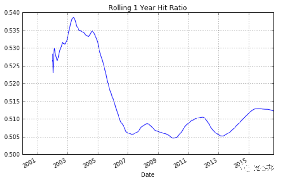

strat['roll12mret'].plot(grid=True, figsize=(8,5),title='Rolling 1 Year Returns')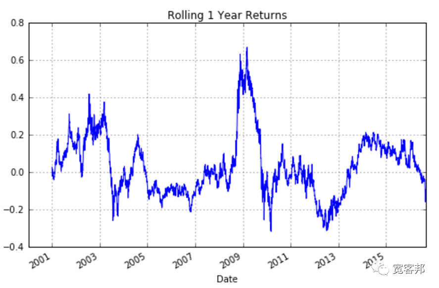

strat['Strategy'].plot(grid=True, figsize=(8,5),title='Daily Returns')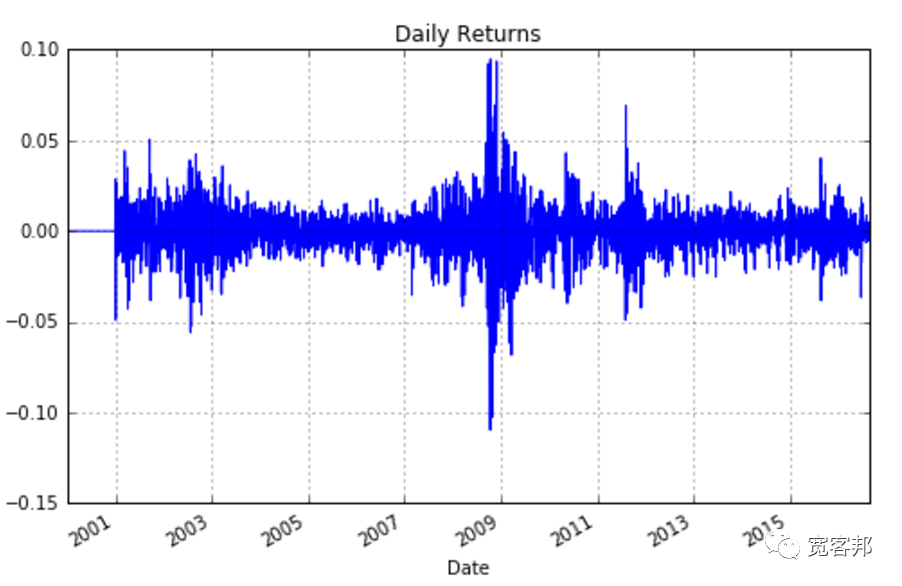

strat['Strategy'].plot(kind='hist',figsize=(8,5),title='Daily Return Distribution',bins=100)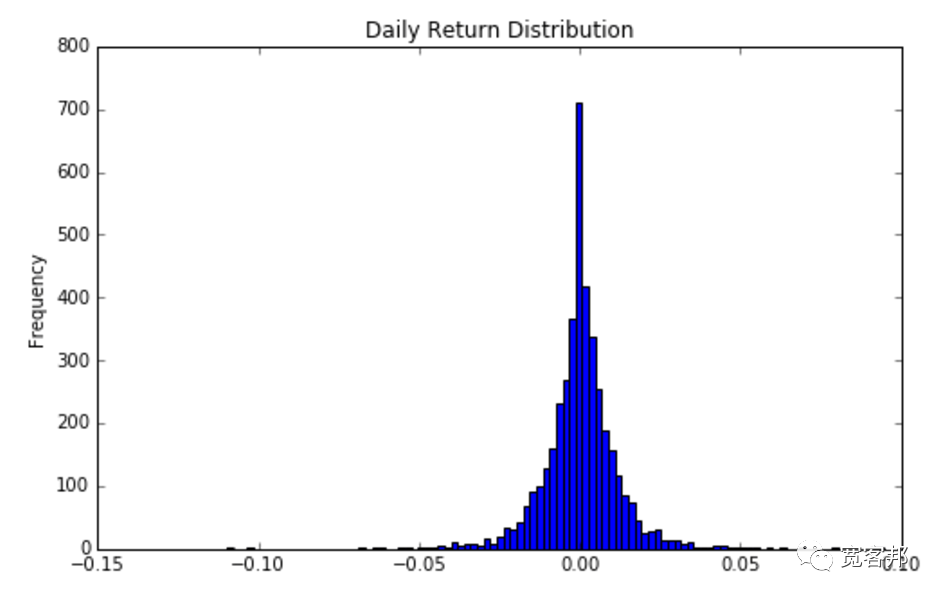

作为旁注，我们可以非常快速地查看每日收益分布的斜率和峰度，如下所示：

print("Skew:",round(strat['Strategy'].skew(),4))print("Kurtosis:",round(strat['Strategy'].kurt(),4))

Skew: 0.0331Kurtosis: 9.4377

因此，每日收益分布与正态分布相差甚远，呈现出略微正偏斜和高峰态（n.b. 正态分布的偏斜为 0，正态分布的峰度为 3）。

在这一点上，我将继续深入挖掘并生成一些关键绩效指标 (KPI)，您通常会在分析任何交易策略回报时找到这些指标。

我们计划生成以下指标：

1) 年化回报

2) 最近 12 个月的回报

3) 波动性

4) 夏普比率

5) 最大回撤

6) Calmar Ratio（年化回报/最大回撤）

7) 波动率/最大跌幅

8) 最佳月度表现

9) 最差月表现

10) 盈利月份的百分比和非盈利月份的百分比

11) 盈利月数/非盈利月数

12) 平均每月利润

13) 平均每月亏损

14) 平均每月利润/平均每月亏损

在我继续之前，我将快速构建另一个新的 DataFrame，它将每月而不是每天保存我们的策略回报数据——这将使稍后的某些计算更容易，并允许我们生成每月回报表。这可以通过“重新采样”每日策略回报的原始 DataFrame 列并从那里建立来产生。

#创建一个新的 DataFrame 来保存我们的每月数据，并使用我们的每日收益列中的数据填充它#original DataFrame 并按月求和stratm = pd.DataFrame(strat['Strategy'].resample('M').sum())
#构建月度数据权益曲线stratm['Strategy Equity'] = stratm['Strategy'].cumsum()+1
#添加一个包含数字月指数的列（即 Jan = 1、Feb = 2 等）stratm['month'] = stratm.index.month

如果我们现在调用函数可以看到每月的DataFrame格式：

stratm.head(15)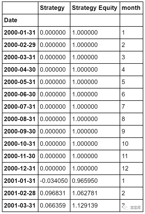

让我们开始研究的 KPI 列表：

#1) 年化回报
days = (strat.index[-1] - strat.index[0]).dayscagr = ((((strat['Strategy Equity'][-1]) / strat['Strategy Equity'][1])) ** (365.0/days)) - 1print('CAGR =',str(round(cagr,4)*100)+"%")

CAGR = 2.28%

#2) 过去 12 个月回报
stratm['last12mret'] = stratm['Strategy'].rolling(window=12,center=False).sum()last12mret = stratm['last12mret'][-1]print('last 12 month return =',str(round(last12mret*100,2))+"%")

过去 12 个月的回报 = -13.14%

#3) 波动率voldaily = (strat['Strategy'].std()) * sqrt(252)volmonthly = (stratm['Strategy'].std()) * sqrt(12)print('Annualised volatility using daily data =',str(round(voldaily,4)*100)+"%")print('Annualised volatility using monthly data =',str(round(volmonthly,4)*100)+"%")

Annualised volatility using daily data = 19.15%<br>Annualised volatility using monthly data = 15.27%

#4) 夏普比率dailysharpe = cagr/voldailymonthlysharpe = cagr/volmonthlyprint('daily Sharpe =',round(dailysharpe,2))print('monthly Sharpe =',round(monthlysharpe,2))

daily Sharpe= 0.12monthly Sharpe= 0.15

#5) 最大回撤
#创建最大回撤函数def max_drawdown(X):    mdd = 0    peak = X[1]for x in X:if x > peak:             peak = x        dd = (peak - x) / peakif dd > mdd:            mdd = ddreturn mdd  


mdd_daily = max_drawdown(strat['Strategy Equity'])mdd_monthly = max_drawdown(stratm['Strategy Equity'])print('max drawdown daily data =',str(round(mdd_daily,4)*100)+"%")print('max drawdown monthly data =',str(round(mdd_monthly,4)*100)+"%")

max drawdown daily data = 37.06%max drawdown monthly data = 33.65%

#6) Calmar比率calmar = cagr/mdd_dailyprint('Calmar ratio =',round(calmar,2))

Calmar ratio = 0.06

#7 波动率/最大回撤vol_dd = volmonthly / mdd_dailyprint('Volatility / Max Drawdown =',round(vol_dd,2))

Volatility/ MaxDrawdown= 0.41

#8) 最佳月度表现bestmonth = max(stratm['Strategy'])print('Best month =',str(round(bestmonth,2))+"%")

Best month = 19.0%

#9) 最差月表现worstmonth = min(stratm['Strategy'])print('Worst month =',str(round(worstmonth,2)*100)+"%")

Worst month = -10.0%

#10) 盈利月份百分比和非盈利月份百分比positive_months = len(stratm['Strategy'][stratm['Strategy'] > 0])negative_months = len(stratm['Strategy'][stratm['Strategy'] < 0])flatmonths = len(stratm['Strategy'][stratm['Strategy'] == 0])perc_positive_months = positive_months / (positive_months + negative_months + flatmonths)perc_negative_months = negative_months / (positive_months + negative_months + flatmonths)print('% of Profitable Months =',str(round(perc_positive_months,2)*100)+"%")print('% of Non-profitable Months =',str(round(perc_negative_months,2)*100)+"%")

% of ProfitableMonths= 49.0%<br>% of Non-profitable Months= 45.0%

#11) 盈利月数/非盈利月数prof_unprof_months = positive_months / negative_monthsprint('Number of Profitable Months/Number of Non Profitable Months',round(prof_unprof_months,2))

Number of ProfitableMonths/Number of NonProfitableMonths1.08

#12) 平均每月利润av_monthly_pos = (stratm['Strategy'][stratm['Strategy'] > 0]).mean()print('Average Monthly Profit =',str(round(av_monthly_pos,4)*100)+"%")
#13) 平均每月损失av_monthly_neg = (stratm['Strategy'][stratm['Strategy'] < 0]).mean()print('Average Monthly Loss =',str(round(av_monthly_neg*100,2))+"%")
#14) pos_neg_month = abs(av_monthly_pos / av_monthly_neg)print('Average Monthly Profit/Average Monthly Loss',round(pos_neg_month,4))

AverageMonthlyProfit= 3.56%<br>AverageMonthlyLoss= -3.33%<br>AverageMonthlyProfit/AverageMonthlyLoss1.0683

最后，为了完成并使用更多的 Pandas DataFrame 功能，我将创建一个每月回报表。

第一步是创建一个数据透视表并对其重新采样以创建所谓的“pandas.tseries.resample.DatetimeIndexResampler”对象。

monthly_table = stratm[['Strategy','month']].pivot_table(stratm[['Strategy','month']], index=stratm.index, columns='month', aggfunc=np.sum).resample('A')

为了让我们可以更轻松地操作它，我将使用“.aggregate()”函数将该对象转换回“DataFrame”。

monthly_table = monthly_table.aggregate('sum')

我们现在可以通过将索引日期转换为仅显示年份而不是完整日期来完成最后的工作，然后还将列月份标题（当前为数字格式）替换为正确的“MMM”格式。

首先，我们必须快速删除表列索引级别之一，当前是“Strategy”一词——这将给我们留下一个表，其中只有一个与整数月份表示相对应的单级别列索引。

#删除当前显示为"Strategy"的顶级列索引monthly_table.columns = monthly_table.columns.droplevel()

从视觉上看，表格将从：

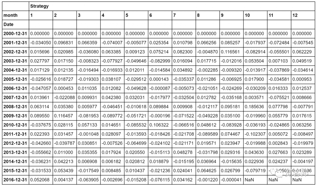
变成：

现在我们只需将日期索引更改为以年度格式 (YYYY) 显示，并将剩余的列标题更改为以月格式 (MMM) 显示。

#仅用相应的年份替换索引列中的完整日期monthly_table.index = monthly_table.index.year
#用 MMM 格式替换整数列标题monthly_table.columns = ['Jan','Feb','Mar','Apr','May','Jun','Jul','Aug','Sep','Oct','Nov','Dec']

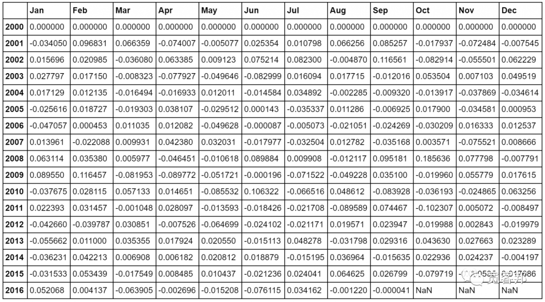
我们现在剩下的每月回报表如下所示：

扫描本文最下方二维码获取全部完整源码和Jupyter Notebook 文件打包下载。

↓↓长按扫码获取完整源码↓↓