图神经网络的可解释性方法介绍和GNNExplainer解释预测的代码示例（附代码）-技术圈

来源：DeepHub IMBA
本文约3800字，建议阅读7分钟
本文使用pytorch-geometric实现的GNNExplainer作为示例。

深度学习模型的可解释性为其预测提供了人类可以理解的推理。如果不解释预测背后的原因，深度学习算法就像黑匣子，对于一些场景说是无法被信任的。不提供预测的原因也会阻止深度学习算法在涉及跨域公平、隐私和安全的关键应用程序中使用。

深度学习模型的可解释性有助于增加对模型预测的信任，提高模型对与公平、隐私和其他安全挑战相关的关键决策应用程序的透明度，并且可以让我们了解网络特征，以便在将模型部署到现实世界之前识别和纠正模型所犯错误的系统模式。

图在现实世界中无处不在，代表社交网络、引用网络、化学分子、金融数据等。图神经网络 (GNN) 是一个强大的框架，用于对图相关数据进行机器学习，例如节点分类、图分类、和链接预测。

所以本文探讨以下5方面：

GNN 需要可解释性
解释 GNN 预测的挑战
不同的 GNN 解释方
GNNExplainer的直观解释
使用 GNNExplainer 解释节点分类和图分类的实现

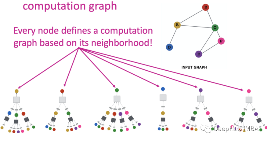
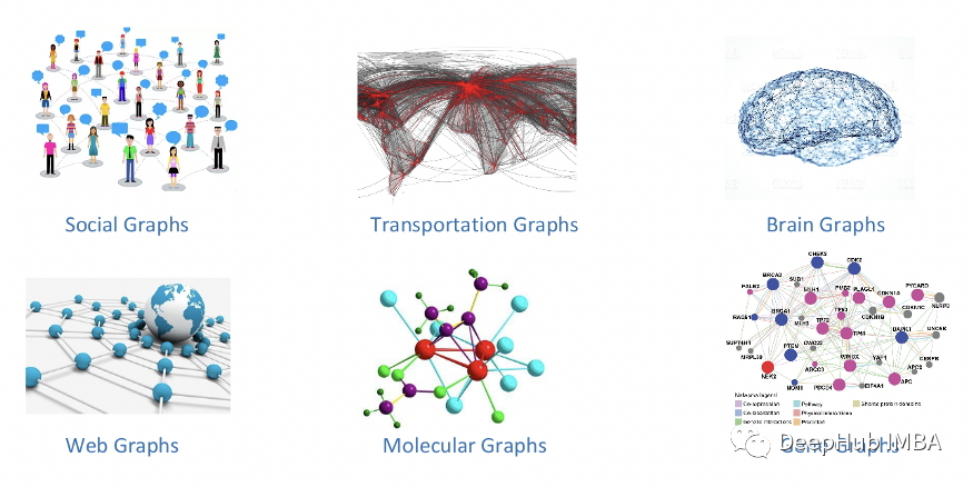
图卷积神经网络 (GCN)、GraphSAGE 和图注意网络 (GAT) 等 GNN 通过沿输入图的边缘递归传递神经消息，将节点特征信息与图结构相结合。

同时结合图结构和特征信息会导致复杂的模型；因此，解释 GNN 的预测是具有挑战性的。

图数据不如图像和文本直观，这使得对图深度学习模型的人类可以理解的解释具有挑战性。
图像和文本使用网格状数据；但是在拓扑图中，信息是使用特征矩阵和邻接矩阵来表示的，每个节点都有不同的邻居。因此图像和文本的可解释性方法不适合获得对图的高质量解释。
图节点和边对 GNN 的最终预测有显着贡献；因此GNN 的可解释性需要考虑这些交互。
节点分类任务通过执行来自其邻居的消息遍历来预测节点的类别。消息游走可以更好地了解 GNN 做出预测的原因，但这与图像和文本相比更具有挑战性。

GNN 解释方法

图可解释性需要回答以下问题：

哪些输入边更关键，对预测贡献最大？
哪些输入节点更重要？
哪些节点特征更重要？
什么图模式将最大化某个类的预测？

解释 GNN 的方法根据它们提供的解释类型分为两个分支。这些图解释方法侧重于图模型的不同方面，并提供不同的视图来理解 GNN 模型。

实例级方法：给定一个输入图，实例级方法通过识别用于预测的重要输入特征来解释深度模型。

模型级方法提供了一般见解和高级理解来解释深度图模型。模型级方法专门研究哪些输入图模式可以导致 GNN 进行某种预测。

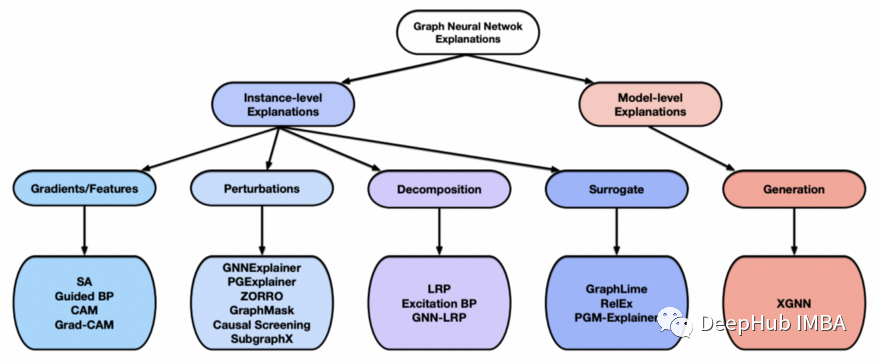
上图为解释 GNN 的不同方法

实例级方法根据重要性分数的获得方式进行区分，可以将它们分为四个不同的分支。

Gradients/Feature-based 方法使用梯度或隐藏特征图来表示不同输入特征的重要性，其中梯度或特征值越高表示重要性越高。基于梯度/特征的可解释性方法广泛用于图像和文本任务。SA、Guided back propagation、CAM 和 Grad-CAM 是基于梯度/特征的可解释性方法的示例。
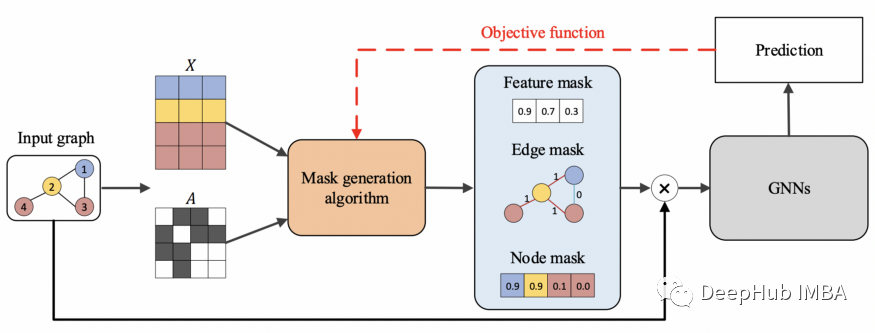
基于扰动的方法监测不同输入扰动的输出变化变化。当保留重要的输入信息时，预测应该与原始预测相似。GNN 可以通过使用不同的掩码生成算法来获得不同类型的掩码来进行特征重要性的判断，如 GNNExplainer、PGExplainer、ZORRO、GraphMask、Causal Screening 和 SubgraphX。
分解方法通过将原始模型预测分解为若干项来衡量输入特征的重要性，这些项被视为相应输入特征的重要性分数。
代理方法采用简单且可解释的代理模型来近似复杂深度模型对输入示例的相邻区域的预测。代理方法包括 GraphLime、RelEx 和 PGM Explainer。

GNNExplainer

GNNExplainer 是一种与模型无关的基于扰动的方法，可以为任何基于图的机器学习任务上的任何基于 GNN 的模型的预测提供可解释的报告。

GNNExplainer 学习边和节点特征的软掩码，然后通过掩码的优化来解释预测。

GNNExplainer 会获取输入图并识别紧凑的子图结构和在预测中起关键作用的一小部分节点特征。

GNNExplainer通过生成传递关键语义的掩码来捕获重要的输入特征，从而产生与原始预测相似的预测。它学习边缘和节点特征的软掩码，通过掩码优化来解释预测。

以不同方式为输入图获得掩码可以获得重要的输入特征。还根据预测任务的类型生成不同的掩码，例如节点掩码、边掩码和节点特征掩码。

生成的掩码与输入图相结合，通过逐元素乘法获得包含重要输入信息的新图。最后，将新图输入经过训练的 GNN 以评估掩码并更新掩码生成算法。

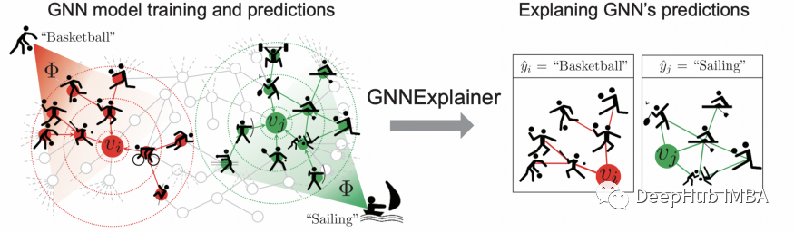
GNNExplainer 示例

explain_node() 学习并返回一个节点特征掩码和一个边缘掩码，它们在解释 GNN 对节点分类所做的预测中起着至关重要的作用。


#Import Library
import numpy as npimport pandas as pdimport osimport torch_geometric.transforms as Tfrom torch_geometric.datasets import Planetoidimport matplotlib.pyplot as pltimport torchimport torch.nn.functional as Ffrom torch_geometric.nn import GCNConv, GNNExplainerimport torch_geometricfrom torch_geometric.loader import NeighborLoaderfrom torch_geometric.utils import to_networkx

#Load the Planetoid datasetdataset = Planetoid(root='.', name="Pubmed")data = dataset[0]
#Set the device dynamicallydevice = torch.device('cuda' if torch.cuda.is_available() else 'cpu')
# Create batches with neighbor samplingtrain_loader = NeighborLoader(  data,  num_neighbors=[5, 10],  batch_size=16,  input_nodes=data.train_mask,)
# Define the GCN modelclass Net(torch.nn.Module):  def __init__(self):      super().__init__()
      self.conv1 = GCNConv(dataset.num_features, 16, normalize=False)      self.conv2 = GCNConv(16, dataset.num_classes, normalize=False)      self.optimizer = torch.optim.Adam(self.parameters(), lr=0.02, weight_decay=5e-4)  def forward(self, x, edge_index):      x = F.relu(self.conv1(x, edge_index))      x = F.dropout(x, training=self.training)      x = self.conv2(x, edge_index)      return F.log_softmax(x, dim=1)
model = Net().to(device)def accuracy(pred_y, y):  """Calculate accuracy."""  return ((pred_y == y).sum() / len(y)).item()
# define the function to Train the modeldef train_nn(model, x,edge_index,epochs):  criterion = torch.nn.CrossEntropyLoss()  optimizer = model.optimizer
  model.train()  for epoch in range(epochs+1):    total_loss = 0    acc = 0    val_loss = 0    val_acc = 0
    # Train on batches    for batch in train_loader:      optimizer.zero_grad()
      out = model(batch.x, batch.edge_index)      loss = criterion(out[batch.train_mask], batch.y[batch.train_mask])
      total_loss += loss      acc += accuracy(out[batch.train_mask].argmax(dim=1),                      batch.y[batch.train_mask])      loss.backward()      optimizer.step()
      # Validation      val_loss += criterion(out[batch.val_mask], batch.y[batch.val_mask])      val_acc += accuracy(out[batch.val_mask].argmax(dim=1),                          batch.y[batch.val_mask])
    # Print metrics every 10 epochs    if(epoch % 10 == 0):        print(f'Epoch {epoch:>3} | Train Loss: {total_loss/len(train_loader):.3f} '              f'| Train Acc: {acc/len(train_loader)*100:>6.2f}% | Val Loss: '              f'{val_loss/len(train_loader):.2f} | Val Acc: '              f'{val_acc/len(train_loader)*100:.2f}%')
# define the function to Test the modeldef test(model, data):  """Evaluate the model on test set and print the accuracy score."""  model.eval()  out = model(data.x, data.edge_index)  acc = accuracy(out.argmax(dim=1)[data.test_mask], data.y[data.test_mask])  return acc

# Train the Modeltrain_nn(model, data.x, data.edge_index, 200)
# Testprint(f'\nGCN test accuracy: {test(model, data)*100:.2f}%\n')
# Explain the GCN for nodenode_idx = 20x, edge_index = data.x, data.edge_index# Pass the model to explain to GNNExplainerexplainer = GNNExplainer(model, epochs=100,return_type='log_prob')#returns a node feature mask and an edge mask that play a crucial role to explain the prediction made by the GNN for node 20node_feat_mask, edge_mask = explainer.explain_node(node_idx, x, edge_index)ax, G = explainer.visualize_subgraph(node_idx, edge_index, edge_mask, y=data.y)plt.show()print("Ground Truth label for node: ",node_idx, " is ", data.y.numpy()[node_idx])out = torch.softmax(model(data.x, data.edge_index), dim=1).argmax(dim=1)print("Prediction for node ",node_idx, "is " ,out[node_idx].cpu().detach().numpy().squeeze())

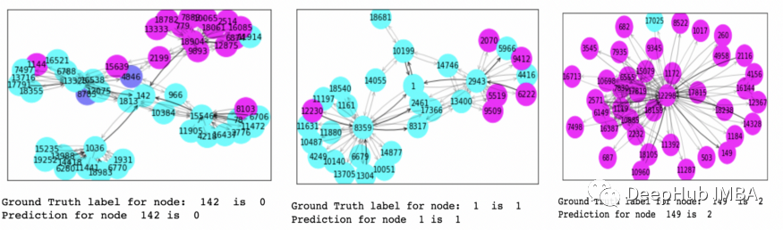
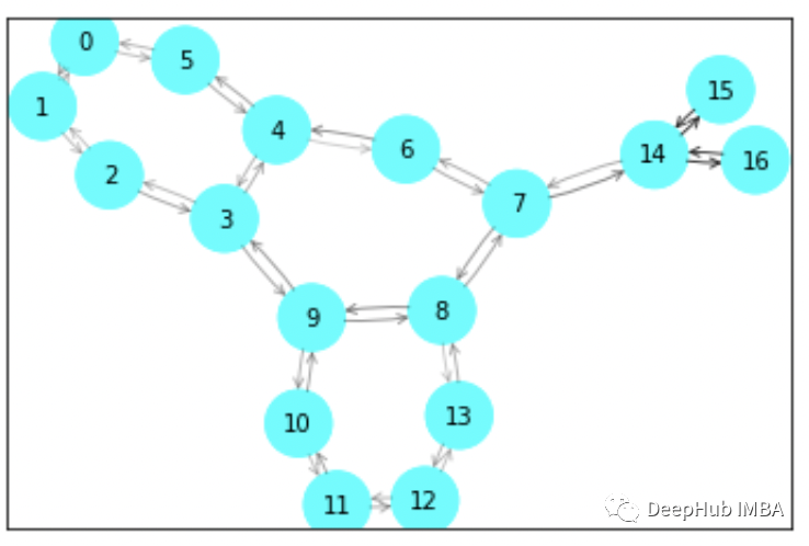
上图中所有颜色相似的节点都属于同一个类。可视化有助于解释哪些节点对预测贡献最大。

Explain_graph()用于图分类;它学习并返回一个节点特征掩码和一个边缘掩码，这两个掩码在解释GNN对一个图的预测时起着至关重要的作用


# Import libarariesimport numpy as npimport pandas as pdimport os
import torch_geometric.transforms as Tfrom torch_geometric.datasets import Planetoidimport matplotlib.pyplot as pltimport torchimport torch.nn.functional as Ffrom torch_geometric.nn import GraphConvimport torch_geometricfrom torch.nn import Parameterfrom torch_geometric.nn.conv import MessagePassingimport urllib.requestimport tarfilefrom torch.nn import Linearimport torch.nn.functional as Ffrom torch_geometric.nn import GCNConv, GNNExplainerfrom torch_geometric.nn import global_mean_poolfrom torch_geometric.datasets import TUDatasetfrom torch_geometric.loader import DataLoader
# Load the datasetdataset = TUDataset(root='data/TUDataset', name='MUTAG')
# print details about the graphprint(f'Dataset: {dataset}:')print("Number of Graphs: ",len(dataset))print("Number of Freatures: ", dataset.num_features)print("Number of Classes: ", dataset.num_classes)
data= dataset[0]print(data)print("No. of nodes: ", data.num_nodes)print("No. of Edges: ", data.num_edges)print(f'Average node degree: {data.num_edges / data.num_nodes:.2f}')print(f'Has isolated nodes: {data.has_isolated_nodes()}')print(f'Has self-loops: {data.has_self_loops()}')print(f'Is undirected: {data.is_undirected()}')
# Create train and test datasettorch.manual_seed(12345)dataset = dataset.shuffle()
train_dataset = dataset[:50]test_dataset = dataset[50:]
print(f'Number of training graphs: {len(train_dataset)}')print(f'Number of test graphs: {len(test_dataset)}')
'''graphs in graph classification datasets are usually small,a good idea is to batch the graphs before inputtingthem into a Graph Neural Network to guarantee full GPU utilization___In pytorch Geometric adjacency matrices are stacked in a diagonal fashion(creating a giant graph that holds multiple isolated subgraphs), and node and target features are simply concatenated in the node dimension:'''

train_loader = DataLoader(train_dataset, batch_size=64, shuffle= True)test_loader= DataLoader(test_dataset, batch_size=64, shuffle= False)
for step, data in enumerate(train_loader):  print(f'Step {step + 1}:')  print('=======')  print(f'Number of graphs in the current batch: {data.num_graphs}')  print(data)  print()
# Build the modelclass GNN(torch.nn.Module):  def __init__(self, hidden_channels):      super(GNN, self).__init__()      torch.manual_seed(12345)      self.conv1 = GraphConv(dataset.num_node_features, hidden_channels)      self.conv2 = GraphConv(hidden_channels, hidden_channels)
      self.conv3 = GraphConv(hidden_channels, hidden_channels )      self.lin = Linear(hidden_channels, dataset.num_classes)
  def forward(self, x, edge_index, batch):      x = self.conv1(x, edge_index)      x = x.relu()      x = self.conv2(x, edge_index)      x = x.relu()      x = self.conv3(x, edge_index)
      x = global_mean_pool(x, batch)
      x = F.dropout(x, p=0.5, training=self.training)      x = self.lin(x)
      return xmodel = GNN(hidden_channels=64)print(model)
# set the optimizeroptimizer = torch.optim.Adam(model.parameters(), lr=0.02)
# set the loss functioncriterion = torch.nn.CrossEntropyLoss()
# Creating the function to train the modeldef train():  model.train()
  for data in train_loader: # Iterate in batches over the training dataset.        out = model(data.x, data.edge_index, data.batch) # Perform a single forward pass.        loss = criterion(out, data.y) # Compute the loss.        loss.backward() # Derive gradients.        optimizer.step() # Update parameters based on gradients.        optimizer.zero_grad() # Clear gradients.
# function to test the modeldef test(loader):    model.eval()
    correct = 0    for data in loader: # Iterate in batches over the training/test dataset.        out = model(data.x, data.edge_index, data.batch)          pred = out.argmax(dim=1) # Use the class with highest probability.        correct += int((pred == data.y).sum()) # Check against ground-truth labels.    return correct / len(loader.dataset) # Derive ratio of correct predictions.
# Train the model for 150 epochsfor epoch in range(1, 160):  train()  train_acc = test(train_loader)  test_acc = test(test_loader)  if(epoch % 10 == 0):        '''print(f'Epoch {epoch:>3} | Train Loss: {total_loss/len(train_loader):.3f} '              f'| Train Acc: {acc/len(train_loader)*100:>6.2f}% | Val Loss: '              f'{val_loss/len(train_loader):.2f} | Val Acc: '              f'{val_acc/len(train_loader)*100:.2f}%')        '''        print(f'Epoch: {epoch:03d}, Train Acc: {train_acc:.4f}, Test Acc: {test_acc:.4f}')
#Explain the Graphexplainer = GNNExplainer(model, epochs=100,return_type='log_prob')data = dataset[0]node_feat_mask, edge_mask = explainer.explain_graph(data.x, data.edge_index)ax, G = explainer.visualize_subgraph(-1,data.edge_index, edge_mask, data.y)plt.show()

当可视化visualize_subgraph时，需要将node_idx设置为-1，因为这意味着一个图分类任务;否则会报错。

本文使用的是pytorch-geometric实现的GNNExplainer作为示例。

有兴趣了解的话可以查看其官方文档

https://pytorch-geometric.readthedocs.io/en/latest/modules/nn.html?highlight=gnnexplainer#torch_geometric.nn.models.GNNExplainer

编辑：于腾凯