基于OpenCV进行车牌检测！-技术圈

转自：小白学视觉

车牌识别及步骤

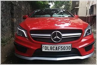
1.车牌检测：第一步是从车上检测车牌。我们将使用OpenCV中的轮廓选项来检测矩形对象以查找车牌。如果我们知道车牌的确切尺寸、颜色和大致位置，可以提高准确度。通常，检测算法是根据特定国家使用的摄像机位置和车牌类型进行训练的。如果图像中甚至没有汽车，这将变得更加棘手，在这种情况下，我们将执行额外的步骤来检测汽车，然后是车牌。

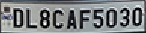
2.字符分割：一旦我们检测到车牌，我们必须将其裁剪出来并保存为新图像。同样，使用OpenCV也可以轻松地完成此操作。

3.字符识别：现在，我们在上一步中获得的新图像肯定会有一些字符（数字/字母）写在上面。因此，我们可以对其执行OCR（光学字符识别）来检测数字。

先决条件：

OpenCV：OpenCV是一个主要针对实时计算机视觉的编程函数库，本项目使用的是4.1.0版。
Python：使用3.6.7版。
IDE：我将在这里使用Jupyter。
Haar cascade：这是一种机器学习对象检测算法，用于识别图像或视频中的对象。
Keras：易于使用并得到广泛支持，Keras使深度学习尽可能简单。
Scikit学习：它是一个用于Python编程语言的自由软件机器学习库。

步骤1　安装依赖库

# installing OpenCV>pip install opencv-python==4.1.0# Installing Keras>pip install keras# Installing Jupyter>pip install jupyter#Installing Scikit-Learn>pip install scikit-learn

步骤2　环境配置

我们将从运行jupyter笔记本开始，然后在我们的案例OpenCV、Keras和sklearn中导入必要的库。

#importing openCV>import cv2#importing numpy>import numpy as np#importing pandas to read the CSV file containing our data>import pandas as pd#importing keras and sub-libraries>from keras.models import Sequential>from keras.layers import Dense>from keras.layers import Dropout>from keras.layers import Flatten, MaxPool2D>from keras.layers.convolutional import Conv2D>from keras.layers.convolutional import MaxPooling2D>from keras import backend as K>from keras.utils import np_utils>from sklearn.model_selection import train_test_split

步骤３　车牌检测

让我们从导入带牌照汽车的示例图像开始，并定义一些函数：

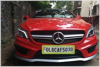
def extract_plate(img): # the function detects and perfors blurring on the number plate.  plate_img = img.copy()    #Loads the data required for detecting the license plates from cascade classifier.  plate_cascade = cv2.CascadeClassifier('./indian_license_plate.xml')
  # detects numberplates and returns the coordinates and dimensions of detected license plate's contours.  plate_rect = plate_cascade.detectMultiScale(plate_img, scaleFactor = 1.3, minNeighbors = 7)
  for (x,y,w,h) in plate_rect:    a,b = (int(0.02*img.shape[0]), int(0.025*img.shape[1])) #parameter tuning    plate = plate_img[y+a:y+h-a, x+b:x+w-b, :]    # finally representing the detected contours by drawing rectangles around the edges.    cv2.rectangle(plate_img, (x,y), (x+w, y+h), (51,51,255), 3)          return plate_img, plate # returning the processed image

上述函数的工作原理是将图像作为输入，然后应用“haar cascade”（经过预训练以检测印度车牌），这里的参数scaleFactor表示一个值，通过该值可以缩放输入图像以更好地检测车牌。minNeighbors只是一个减少误报的参数，如果该值较低，算法可能更容易给出错误识别的输出。

步骤4　车牌图像预处理

现在，让我们进一步处理此图像，以简化角色提取过程。我们将首先为此定义更多函数。

# Find characters in the resulting imagesdef segment_characters(image) :
    # Preprocess cropped license plate image    img = cv2.resize(image, (333, 75))    img_gray = cv2.cvtColor(img, cv2.COLOR_BGR2GRAY)    _, img_binary = cv2.threshold(img_gray, 200, 255, cv2.THRESH_BINARY+cv2.THRESH_OTSU)    img_erode = cv2.erode(img_binary, (3,3))    img_dilate = cv2.dilate(img_erode, (3,3))
    LP_WIDTH = img_dilate.shape[0]    LP_HEIGHT = img_dilate.shape[1]
    # Make borders white    img_dilate[0:3,:] = 255    img_dilate[:,0:3] = 255    img_dilate[72:75,:] = 255    img_dilate[:,330:333] = 255
    # Estimations of character contours sizes of cropped license plates    dimensions = [LP_WIDTH/6, LP_WIDTH/2, LP_HEIGHT/10, 2*LP_HEIGHT/3]
    # Get contours within cropped license plate    char_list = find_contours(dimensions, img_dilate)
    return char_list

上述函数接收图像作为输入，并对其执行以下操作：

将其调整为一个维度，使所有字符看起来清晰明了。
将彩色图像转换为灰度图像，即代替3个通道（BGR），图像只有一个8位通道，其值范围为0–255，其中0对应于黑色，255对应于白色。我们这样做是为了为下一个过程准备图像。
该图像现在是二进制形式，并准备好进行下一个进程侵蚀。
侵蚀是一个简单的过程，用于从对象边界移除不需要的像素，这意味着像素的值应为0，但其值为1。
下一步是使图像的边界变白。
我们已将图像还原为经过处理的二值图像，并准备将此图像传递给字符提取。

步骤5　从车牌中分割字母数字字符

import numpy as npimport cv2
# Match contours to license plate or character templatedef find_contours(dimensions, img) :
    # Find all contours in the image    cntrs, _ = cv2.findContours(img.copy(), cv2.RETR_TREE, cv2.CHAIN_APPROX_SIMPLE)
    # Retrieve potential dimensions    lower_width = dimensions[0]    upper_width = dimensions[1]    lower_height = dimensions[2]    upper_height = dimensions[3]    
    # Check largest 5 or  15 contours for license plate or character respectively    cntrs = sorted(cntrs, key=cv2.contourArea, reverse=True)[:15]
    x_cntr_list = []    target_contours = []    img_res = []    for cntr in cntrs :        #detects contour in binary image and returns the coordinates of rectangle enclosing it        intX, intY, intWidth, intHeight = cv2.boundingRect(cntr)                #checking the dimensions of the contour to filter out the characters by contour's size        if intWidth > lower_width and intWidth < upper_width and intHeight > lower_height and intHeight < upper_height :            x_cntr_list.append(intX) #stores the x coordinate of the character's contour, to used later for indexing the contours
            char_copy = np.zeros((44,24))            #extracting each character using the enclosing rectangle's coordinates.            char = img[intY:intY+intHeight, intX:intX+intWidth]            char = cv2.resize(char, (20, 40))
            # Make result formatted for classification: invert colors            char = cv2.subtract(255, char)
            # Resize the image to 24x44 with black border            char_copy[2:42, 2:22] = char            char_copy[0:2, :] = 0            char_copy[:, 0:2] = 0            char_copy[42:44, :] = 0            char_copy[:, 22:24] = 0
            img_res.append(char_copy) #List that stores the character's binary image (unsorted)
    #Return characters on ascending order with respect to the x-coordinate (most-left character first)        #arbitrary function that stores sorted list of character indeces    indices = sorted(range(len(x_cntr_list)), key=lambda k: x_cntr_list[k])    img_res_copy = []    for idx in indices:        img_res_copy.append(img_res[idx])# stores character images according to their index    img_res = np.array(img_res_copy)
    return img_res

在第4步之后，我们应该有一个干净的二进制图像来处理。在这一步中，我们将应用更多的图像处理来从车牌中提取单个字符。

步骤6　创建机器学习模型并训练模型

数据是干净和准备好的，现在是时候创建一个神经网络，它将足够智能，在训练后识别字符。
对于建模，我们将使用具有3层的卷积神经网络。

## create model>model = Sequential()>model.add(Conv2D(filters=32, kernel_size=(5,5), input_shape=(28, 28, 1), activation='relu'))>model.add(MaxPooling2D(pool_size=(2, 2)))>model.add(Dropout(rate=0.4))>model.add(Flatten())>model.add(Dense(units=128, activation='relu'))>model.add(Dense(units=36, activation='softmax'))

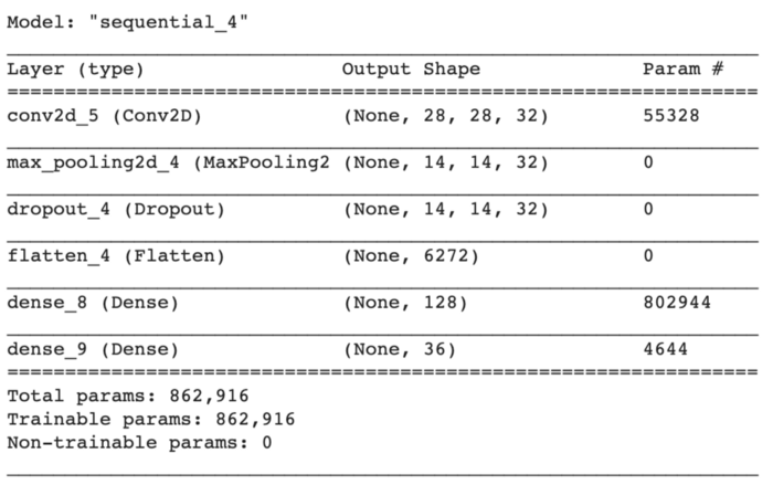
为了保持模型简单，我们将从创建一个顺序对象开始。
第一层是卷积层，具有32个输出滤波器、大小为（5,5）的卷积窗口和“Relu”作为激活函数。
接下来，我们将添加一个窗口大小为（2,2）的最大池层。
最大池是一个基于样本的离散化过程。目标是对输入表示（图像、隐藏层输出矩阵等）进行下采样，降低其维数，并允许对包含在分块子区域中的特征进行假设。
Dropout是一个正则化超参数，用于初始化以防止神经网络过度拟合。辍学是一种在训练过程中忽略随机选择的神经元的技术。他们是随机“退出”的。
现在是展平节点数据的时候了，所以我们添加了一个展平层。展平层从上一层获取数据，并以单个维度表示。
最后，我们将添加两个密集层，一个是输出空间的维数为128，激活函数为'relu'，另一个是我们的最后一个层，有36个输出，用于对26个字母（A-Z）+10个数字（0-9）进行分类，激活函数为'softmax'

步骤7　训练CNN模型

我们将使用的数据包含大小为28x28的字母（A-Z）和数字（0-9）的图像，而且数据是平衡的，因此我们不必在这里进行任何类型的数据调整。
我们将使用“分类交叉熵”作为损失函数，“Adam”作为优化函数，“精度”作为误差矩阵。

import datetimeclass stop_training_callback(tf.keras.callbacks.Callback):  def on_epoch_end(self, epoch, logs={}):    if(logs.get('val_acc') > 0.992):      self.model.stop_training = True      log_dir="logs/fit/" + datetime.datetime.now().strftime("%Y%m%d-%H%M%S")tensorboard_callback = tf.keras.callbacks.TensorBoard(log_dir=log_dir, histogram_freq=1)
batch_size = 1callbacks = [tensorboard_callback, stop_training_callback()]model.fit_generator(train_generator,      steps_per_epoch = train_generator.samples // batch_size,      validation_data = validation_generator,       validation_steps = validation_generator.samples // batch_size,      epochs = 80, callbacks=callbacks)

经过23个阶段的训练，模型的准确率达到99.54%。

步骤8　输出

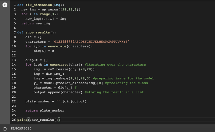
最后，让我们将图像输入到我们的模型中。

往期精彩：

时隔一年！深度学习语义分割理论与代码实践指南.pdf第二版来了！

基于 docker 和 Flask 的深度学习模型部署！

新书预告 | 《机器学习公式推导与代码实现》出版在即！