
7个步骤详解AdaBoost 算法原理和构建流程(附代码)

来源:DeepHub IMBA 本文约6000字,建议阅读10+分钟 本文以简单的数据集为例,为你讲解AdaBoost算法的工作原理。
import pandas as pddf = pd.read_csv("<https://archive.ics.uci.edu/ml/machine-learning-databases/adult/adult.data>",names = ["age","workclass","fnlwgt","education","education-num","marital-status","occupation","relationship","race","sex","capital-gain","capital-loss","hours-per-week","native-country","income"],index_col=False)
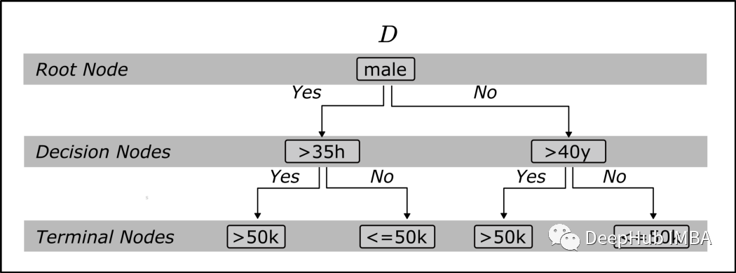
性别:男(是或否) 每周工作时间:>40 小时(是或否) 年龄:>50 (是或否)
import numpy as np# define input parameterdf['male'] = df['sex'].apply(lambda x : 'Yes' if x.lstrip() == "Male" else "No")df['>40 hours'] = np.where(df['hours-per-week']>40, 'Yes', 'No')df['>50 years'] = np.where(df['age']>50, 'Yes', 'No')# targetdf['>50k income'] = df['income'].apply(lambda x : 'Yes' if x.lstrip() == '>50K' else "No")# define datasetdf_simpl = df[['male', '>40 hours','>50 years','>50k income']]df_simpl = df_simpl.head(10)df_simpl
一、构建第一个弱学习者:找到性能最好的“树桩”
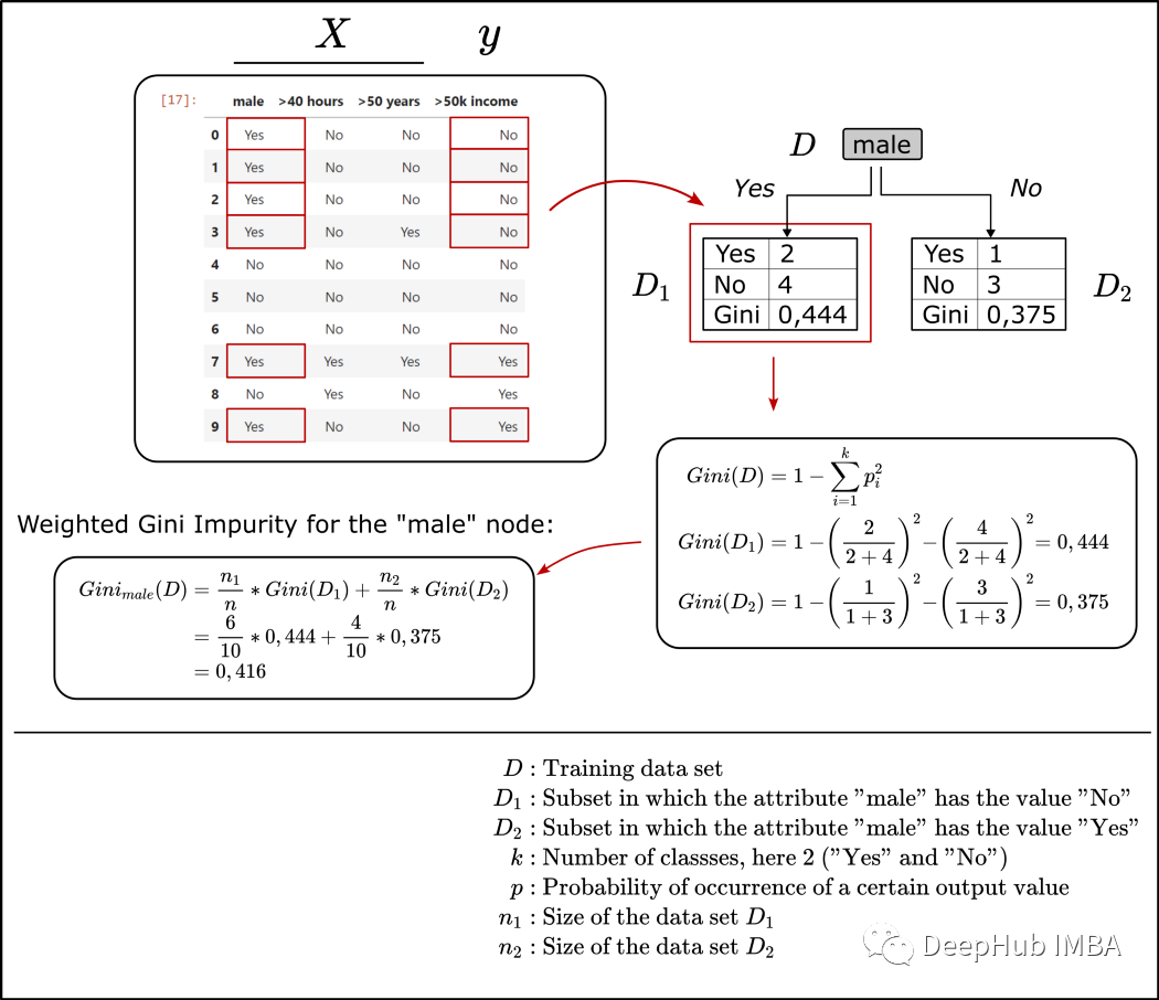
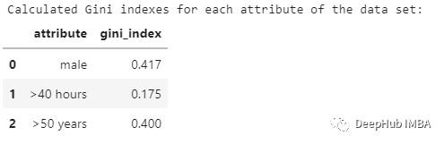
def calc_weighted_gini_index(attribute, df):'''Args:df: the trainings dataset stored in a data frameattribute: the chosen attribute for the root node of the treeReturn:Gini_attribute: the gini index for the chosen attribute'''d_node = df[[attribute, '>50k income']]# number of records in the dataset (=10, for the simple example)n = len(d_node)# number of values "Yes" and "No" for the target variable ">50k income" in the root noden_1 = len(d_node[d_node[attribute] == 'Yes'])n_2 = len(d_node[d_node[attribute] == 'No'])# count "Yes" and "No" values for the target variable ">50k income" in each leafe# left leafe, D_1n_1_yes = len(d_node[(d_node[attribute] == 'Yes') & (d_node[">50k income"] == 'Yes')])n_1_no = len(d_node[(d_node[attribute] == 'Yes') & (d_node[">50k income"] == 'No')])# right leafe, D_2n_2_yes = len(d_node[(d_node[attribute] == 'No') & (d_node[">50k income"] == 'Yes')])n_2_no = len(d_node[(d_node[attribute] == 'No') & (d_node[">50k income"] == 'No')])# Gini index of the left leafeGini_1 = 1-(n_1_yes/(n_1_yes + n_1_no)) ** 2-(n_1_no/(n_1_yes + n_1_no)) ** 2# Gini index of the right leafeGini_2 = 1-(n_2_yes/(n_2_yes + n_2_no)) ** 2-(n_2_no/(n_2_yes + n_2_no)) ** 2# weighted Gini index for the selected feature (=attribute) as root nodeGini_attribute = (n_1/n) * Gini_1 + (n_2/n) * Gini_2Gini_attribute = round(Gini_attribute, 3)print(f'Gini_{attribute} = {Gini_attribute}')return Gini_attributedef find_attribute_that_shows_the_smallest_gini_index(df):'''Args:df: the trainings dataset stored in a data frameReturn:selected_root_node_attribute: the attribute/feature that showed the lowest gini index'''# calculate gini index for each attribute in the dataset and store them in a listattributes = []gini_indexes = []for attribute in df.columns[:-1]:# calculate gini index for attribute as root note using the defined function "calc_weighted_gini_index"gini_index = calc_weighted_gini_index(attribute, df)attributes.append(attribute)gini_indexes.append(gini_index)# create a data frame using the just calculated gini index for each feature/attribute of the datasetprint("Calculated Gini indexes for each attribute of the data set:")d_calculated_indexes = {'attribute':attributes,'gini_index':gini_indexes}d_indexes_df = pd.DataFrame(d_calculated_indexes)display(d_indexes_df)# Find the attribute for the first stump, the attribute where the Gini index is lowest the thus the Gini gain is highest")selected_root_node_attribute = d_indexes_df.min()["attribute"]print(f"Attribute for the root node of the stump: {selected_root_node_attribute}")return selected_root_node_attribute################################################################################################################# to build the first stump we are using the orginial dataset as the train dataset# the defined functions identify the features with the highest Gini gain################################################################################################################df_step_1 = df_simplselected_root_node_attribute = find_attribute_that_shows_the_smallest_gini_index(df_step_1)
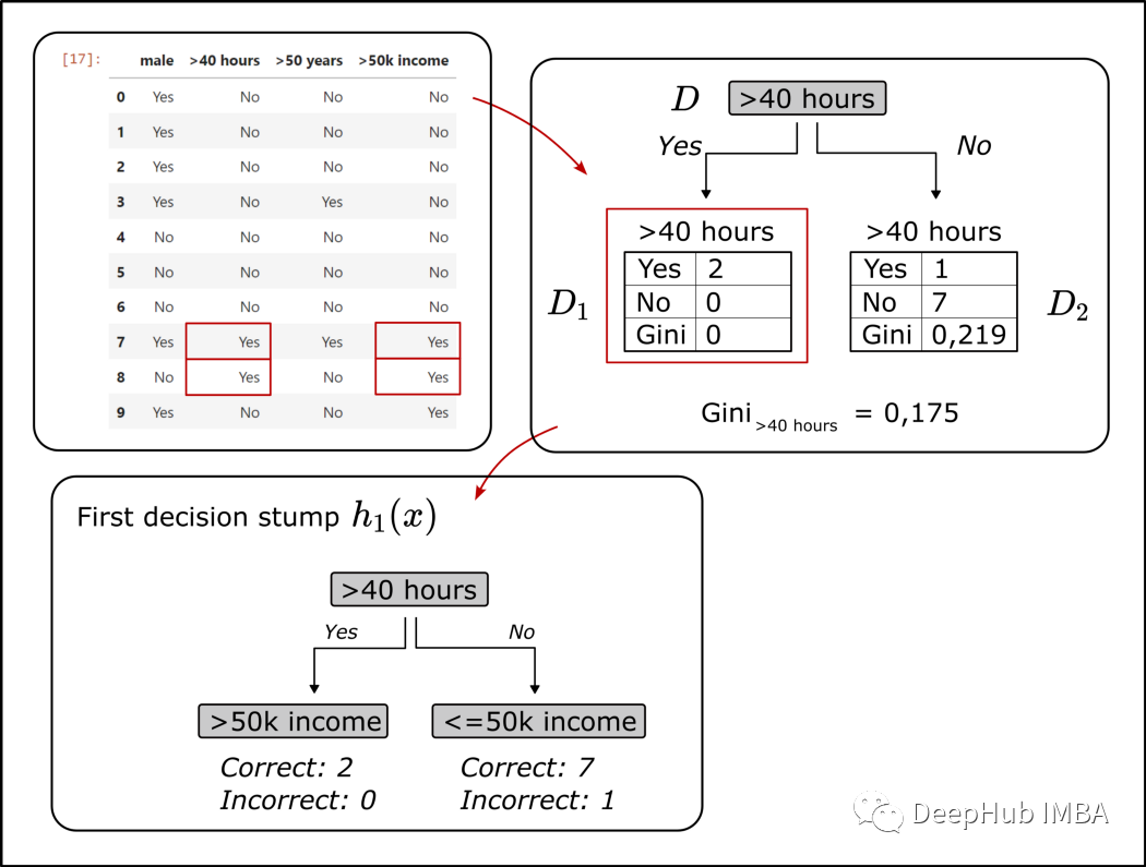
二、计算“树桩”的误差
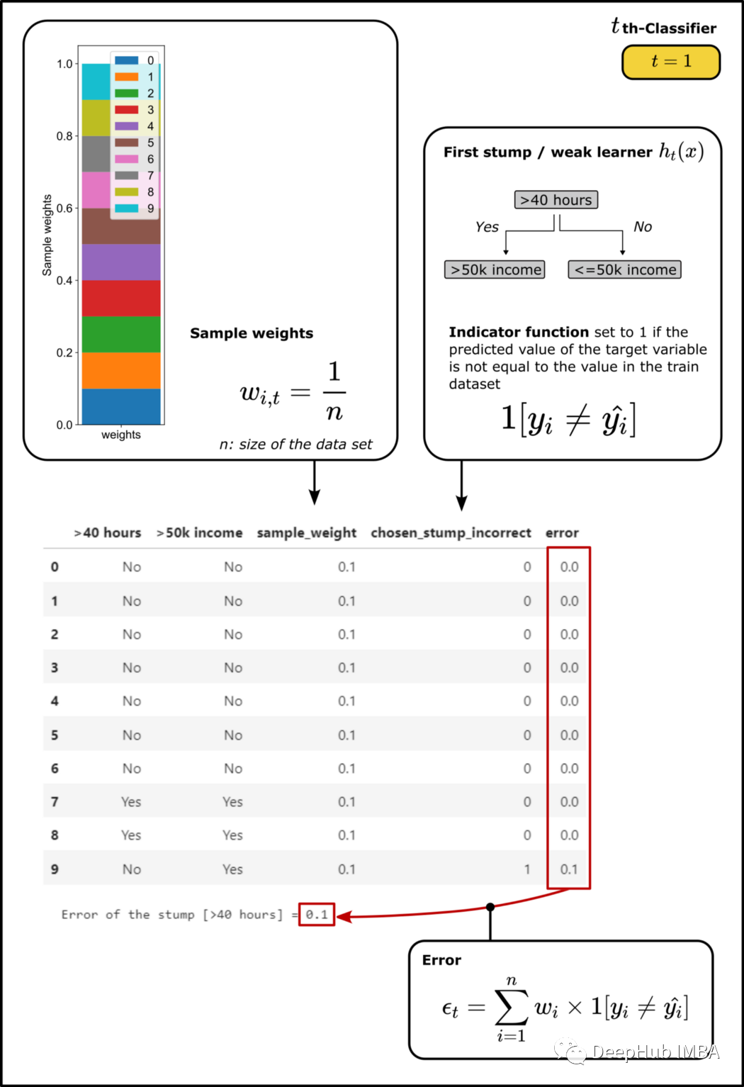
import helper_functionsdef calculate_error_for_chosen_stump(df, selected_root_node_attribute):'''Attributes:df: trainings data setselected_root_node_attribute: name of the column used for the root node of the stumpReturn:df_extended: df extended by the calculated weights and errorerror: calculated error for the stump - sum of the weights of all samples that were misclassified by the decision stub'''# add column for the sample weight, for the first step its simply defined as 1/n, so the sum of all weights is 1df["sample_weight"] = 1/len(df)df[selected_root_node_attribute]df[">50k income"]# in binary classification, we have two ways to build the tree.# (1) That attribute and target value show the same value or# (2) attribute and target value show the opposite value# we choose the one which shows less errors# stump_1_incorrect_v1 and stump_1_incorrect_v2 shows the prediction result of the two stumpsdf["stump_1_incorrect_v1"] = np.where(((df[selected_root_node_attribute] == "Yes") & (df[">50k income"] == "Yes")) |((df[selected_root_node_attribute] == "No") & (df[">50k income"] == "No")),0,1)df["stump_1_incorrect_v2"] = np.where(((df[selected_root_node_attribute] == "Yes") & (df[">50k income"] == "No")) |((df[selected_root_node_attribute] == "No") & (df[">50k income"] == "Yes")),0,1)# select the stump with fewer samples misclassifiedif sum(df['stump_1_incorrect_v1']) <= sum(df["stump_1_incorrect_v2"]):df["chosen_stump_incorrect"] = df['stump_1_incorrect_v1']else:df["chosen_stump_incorrect"] = df['stump_1_incorrect_v2']# drop the columns for the two versions of the treedf = df.drop(['stump_1_incorrect_v1', 'stump_1_incorrect_v2'], axis=1)# calculate the error by multiplying sample weight and the column chosen_stump_incorrectdf["error"] = df["sample_weight"] * df["chosen_stump_incorrect"]error = sum(df["error"])# data frame extended by the weights, errors, etc.df_extended = df# display extended datasetdisplay(df_extended[[selected_root_node_attribute,">50k income","sample_weight", "chosen_stump_incorrect", "error"]])# plot calculated weights in a stacked bar-plothelper_functions.plot_weights(df_extended)print(f'Error of the stump [{selected_root_node_attribute}] = {error}')return df_extended, error# call function to calculate the weighted error for the selected stumpdf_extended_1, error = calculate_error_for_chosen_stump(df_step_1, selected_root_node_attribute)
三、计算“树桩”的权重,也就是“发言权”
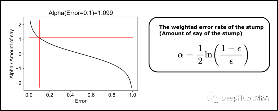
import matplotlib.pyplot as pltfrom datetime import datetime# calculate the amount of say using the weighted error rate of the weak classifieralpha = 1/2 * np.log((1-error)/error)print(f'Amount of say / Alpha = {round(alpha,3)}')helper_functions.plot_alpha(alpha, error)
四、调整样本权重
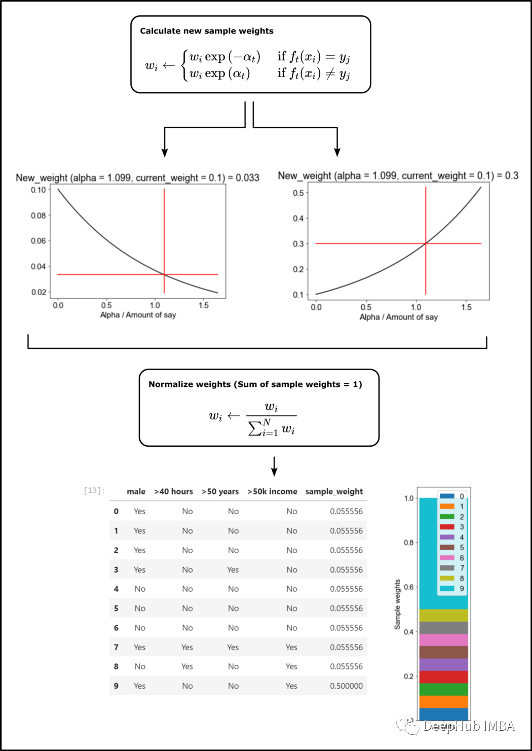
import mathdef plot_scale_of_weights(alpha, current_sample_weight, incorrect):alpha_list = []new_weights = []if incorrect == 1:# adjust the sample weights for instances which were misclassifiednew_weight = current_sample_weight * math.exp(alpha)# calculate x and y for plot of the scaling function and new sample weightfor alpha_n in np.linspace(0, alpha * 1.5, num=100):scale = current_sample_weight * math.exp(alpha_n)alpha_list.append(alpha_n)new_weights.append(scale)else:# adjust the sample weights for instances which were classified correctnew_weight = current_sample_weight * math.exp(-alpha)# calculate x and y for plot of the scaling function and new sample weightfor alpha_n in np.linspace(0, alpha * 1.5, num=100):scale = current_sample_weight * math.exp(-alpha_n)alpha_list.append(alpha_n)new_weights.append(scale)####################################################################################################### plot scaling of the sample weight####################################################################################################### change font size for matplotlib graphfont = {'family': 'arial','weight': 'normal','size': 15}plt.rc('font', **font)plt.plot(alpha_list, new_weights, color='black')plt.plot(np.linspace(alpha, alpha, num=100), new_weights, color='red')plt.plot(np.linspace(0, alpha * 1.5, num=100), np.linspace(new_weight, new_weight, num=100), color='red')plt.xlabel('Alpha / Amount of say')plt.title(f'New_weight (alpha = {round(alpha, 3)}, current_weight = {round(current_sample_weight, 3)}) = {round(new_weight, 3)}')# define plot name and save the figure# datetime object containing current date and timenow = datetime.now()# use timestamp for file name# dd/mm/YY H:M:Sdt_string = now.strftime("%d_%m_%Y_%H_%M_%S")plt.savefig(r'.\\plots\\sample_weights_' + dt_string + '.svg')plt.show()return new_weightnew_weight = plot_scale_of_weights(alpha, current_sample_weight=0.1, incorrect=1)
使用上面定义的函数来更新样本权重:
def update_sample_weights(df_extended_1):# calculate the new weights for the misclassified samplesdef calc_new_sample_weight(x, alpha):new_weight = plot_scale_of_weights(alpha, x["sample_weight"], x["chosen_stump_incorrect"])return new_weightdf_extended_1["new_sample_weight"] = df_extended_1.apply(lambda x: calc_new_sample_weight(x, alpha), axis=1)# define new extended data framedf_extended_2 = df_extended_1[["male", ">40 hours", ">50 years", ">50k income", "new_sample_weight"]]df_extended_2 = df_extended_2.rename(columns={"new_sample_weight": "sample_weight"}, errors="raise")# normalize weightsdf_extended_2["sample_weight"] = df_extended_2["sample_weight"] * 1/df_extended_2["sample_weight"].sum()df_extended_2["sample_weight"].sum()return df_extended_2df_extended_2 = update_sample_weights(df_extended_1)
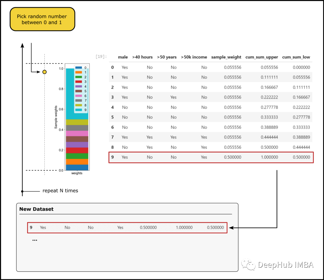
五、第二次运行:形成一个新的自举数据集
计算所有特征的基尼系数,选择特征作为第二个“树桩”的根节点; 建造第二个树桩; 将加权误差计算为误分类样本的样本权重之和。
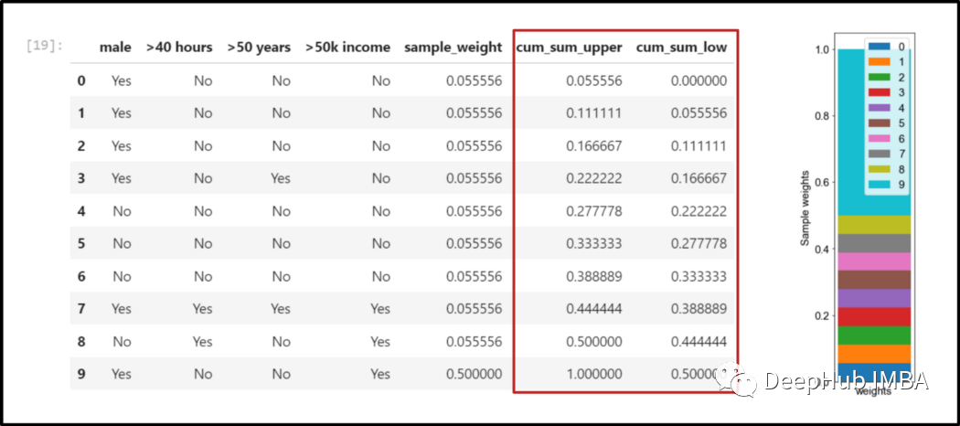
##################################################################################### define bins to select new instances####################################################################################import randomdf_extended_2["cum_sum_upper"] = df_extended_2["sample_weight"].cumsum()df_extended_2["cum_sum_low"] = [0] + df_extended_2["cum_sum_upper"][0:9].to_list()##################################################################################### create new dataset####################################################################################new_data_set = []for i in range(0,len(df_extended_2),1):random_number = random.randint(0, 100)*0.01if i == 0:picked_instance = df_extended_2[(df_extended_2["cum_sum_low"]<random_number) & (df_extended_2["cum_sum_upper"]>random_number)]new_data_set = picked_instanceelse:picked_instance = df_extended_2[(df_extended_2["cum_sum_low"]<random_number) & (df_extended_2["cum_sum_upper"]>random_number)]new_data_set = pd.concat([new_data_set, picked_instance], ignore_index=True)new_data_set
df_step_2 = new_data_set[["male", ">50 years", ">50k income"]]selected_root_node_attribute_2 = find_attribute_that_shows_the_smallest_gini_index(df_step_2)六、重复这个过程,直到达到终止条件
找到最大化基尼收益的弱学习器 h_t(x)(或者最小化错误分类实例的误差)。 将弱学习器的加权误差计算为错误分类样本的样本权重之和。 将分类器添加到集成模型中。模型的结果是对各个弱学习器结果的总结。使用上面确定的“发言权重”/加权错误率 (alpha) 对弱学习者进行加权。 更新发言权重:在加权和误差的帮助下,将 alpha 计算为刚刚形成的弱学习器的“发言权重”。 使用这个 alpha 来重新调整样本权重。 新的样本权重被归一化,使权重之和为 1 使用新的权重,通过在 0 和 1 之间选择一个随机数 N 次来生成一个新的数据集,然后将数据样本添加到表示该数据集的新数据集中。 通过新数据集训练新的弱学习器(与步骤1相同)。
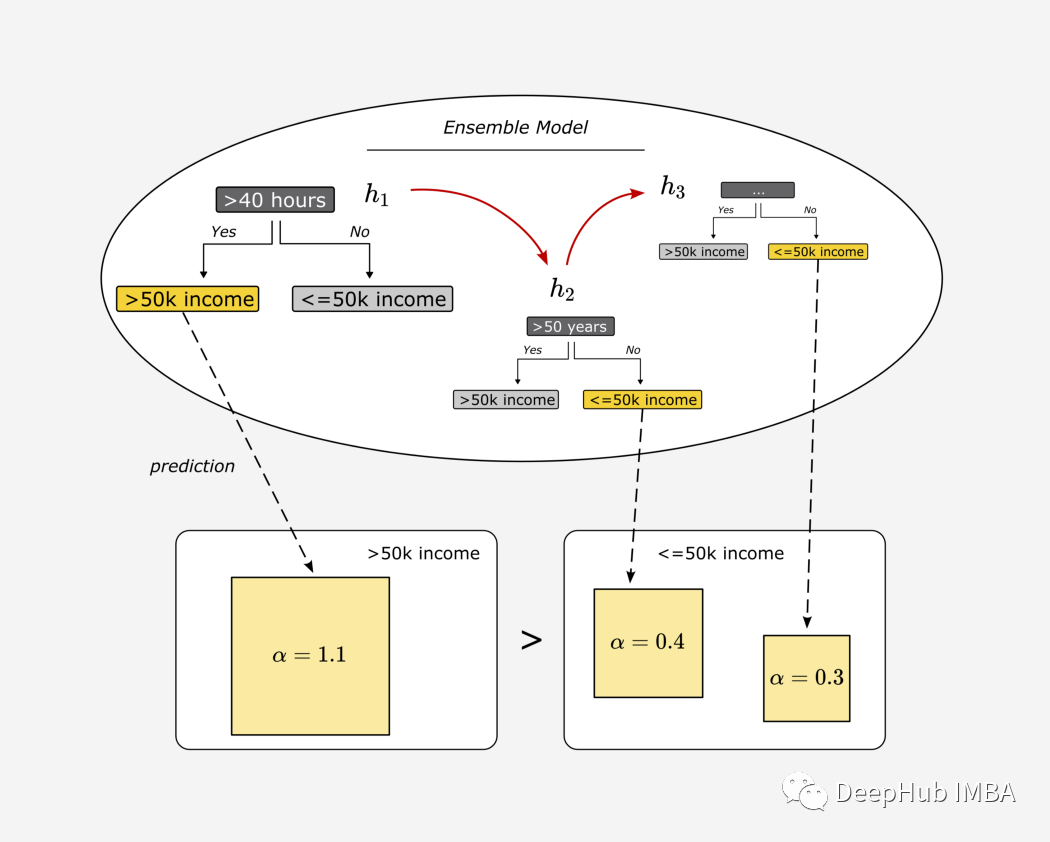
七、将弱学习器组合成一个集成模型
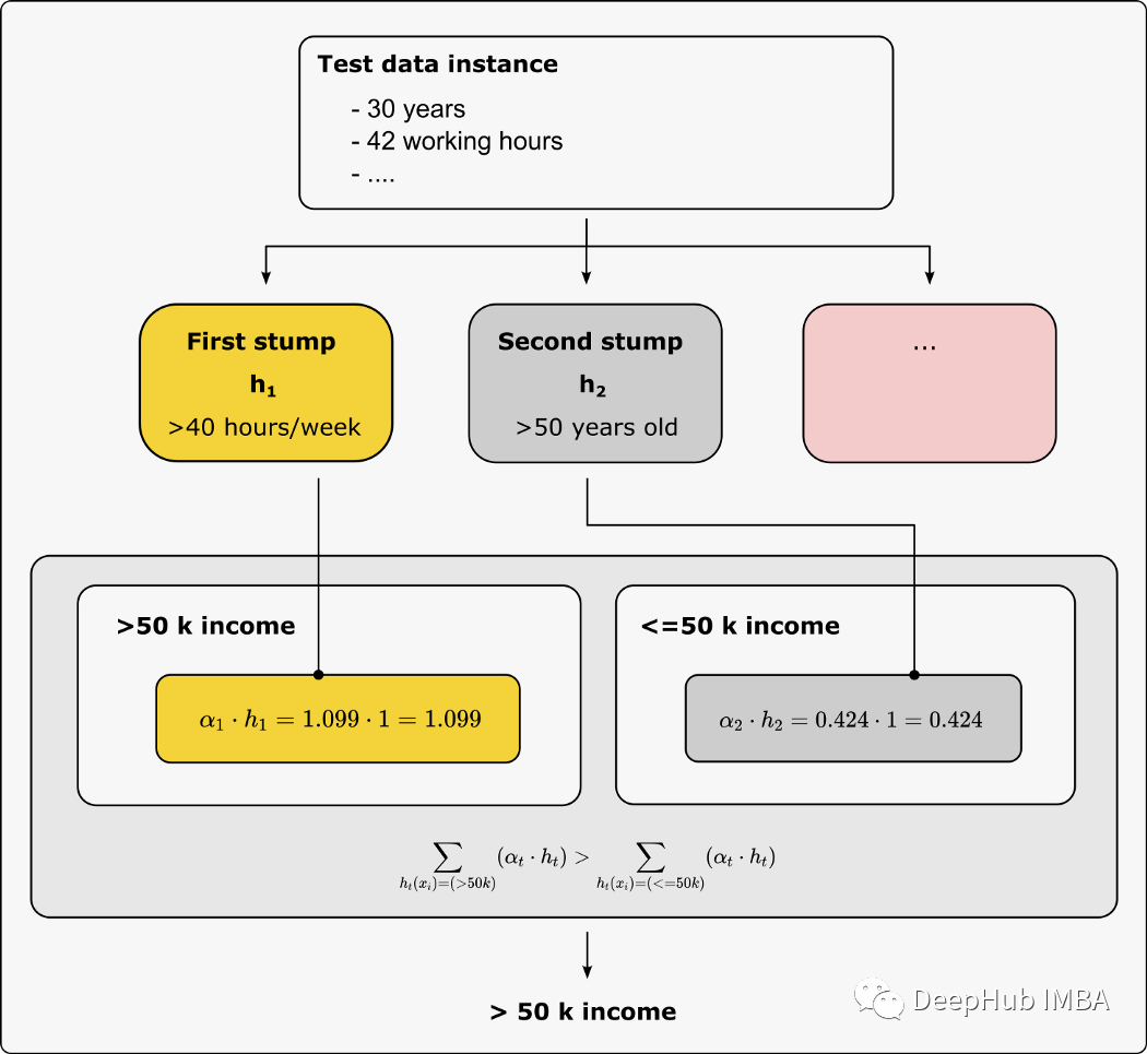
alpha_step_1 = alphaprint(f"Amount of say for the first stump: {round(alpha_step_1,3)}")alpha_step_2 = alpha_step_2print(f"Amount of say for the second stump: {round(alpha_step_2,3)}")########################################################################################### Make a prediction:# Suppose a person lives in the U.S., is 30 years old, and works about 42 hours per week.########################################################################################### the first stump uses the hours worked per week (>40 hours) as the root node# if the regular working hours per week is above 40 hours, the stump would say that the person earns more than 50 k# otherwise, the income would be classified as below 50 kF_1 = 1# the second stump uses the age (>50 years) as root node# if you are over 50 years old, you are more likely to have an income of more than 50 k# in this case, our second weak learner would classifier the target variable (>50 k income) as a 'Yes' or 1# otherwise as a 'No' or 0F_2 = 0# calculate the result of the ensemble modelF_over_50_k = alpha_step_1 * 1 + alpha_step_2 * 0F_below_50_k = alpha_step_1 * 0 + alpha_step_2 * 1if F_over_50_k > F_below_50_k:print("The person has an income of more than 50 k")else:print("The person has an income below 50 k")

总结
编辑:黄继彦
校对:林亦霖
评论