
在TensorFlow中实现胶囊网络
点击上方“小白学视觉”,选择加"星标"或“置顶”
重磅干货,第一时间送达
我们都知道,在许多计算机视觉任务中,卷积神经网络(CNN)的性能均优于人类。所有基于CNN的模型都具有与卷积层相同的基本体系结构,其后是具有中间批处理归一化层的池化层,用于在前向遍历中对批次进行归一化并在后向遍历中控制梯度。
然而,在CNN中,使用最大池化层有几个缺点,因为它没有考虑具有最大值的像素与其直接相邻像素之间的关系。为了解决该问题,Hinton提出了胶囊网络的思想和一种称为“胶囊之间的动态路由”的算法。这篇文章中,我们将介绍该模型的实现细节。
TensorFlow操作
在TensorFlow 2.3中使用功能API或顺序模型构建模型非常容易,只需很少的代码行。但是,在此胶囊网络的实现中,我们利用Functional API和一些自定义操作,并使用@tf.function修饰它们以进行优化。在本节中,将重点介绍tf.matmul较大尺寸的功能。
tf.matmul
对于2D矩阵,只要遵守形状符号,matmul操作即可执行矩阵乘法操作。但是,对于秩为(r> 2)的张量,该运算变为2个运算的组合,即逐元素乘法和矩阵乘法。
对于秩(r = 4)的矩阵,它首先沿轴= [0,1]进行传播(broadcasring),并使它们的形状相同。并且仅当第一个张量的最后一个维度和第二个张量的第二个至最后一个维度具有匹配的维度时,最后两个轴([2,3])才会进行矩阵乘法。为了简洁起见,下面的示例将对其进行说明,为简便起见,仅输出形状,但可以在控制台上随意输出并计算数字。
>>> w = tf.reshape(tf.range(48), (1,8,3,2))>>> x = tf.reshape(tf.range(40), (5,1,2,4))>>> tf.matmul(w, x).shapeTensorShape([5, 8, 3, 4])
w沿轴= 0广播,x沿轴= 1广播,其余两个维矩阵相乘。让我们检查一下matmul的transpose_a / transpose_b参数。在张量上调用tf.transpose时,所有尺寸都将反转。例如,
>>> a = tf.reshape(tf.range(48), (1,8,3,2))>>> tf.transpose(a).shapeTensorShape([2, 3, 8, 1])
因此,让我们看看它是如何工作的 tf.matmul
>>> w = tf.ones((1,10,16,1))>>> x = tf.ones((1152,1,16,1))>>> tf.matmul(w, x, transpose_a=True).shapeTensorShape([1152, 10, 1, 1])
TensorFlow所做的工作首先是沿前两个维度广播,然后将它们假定为2D矩阵堆栈。您可以将其可视化为仅应用于第一个数组的最后两个维度的转置。转置操作后的第一个数组的形状为[1152、10、1、16](将转置应用于最后一个二维),现在应用矩阵乘法。顺便说一下,transpose_a = True将上述转置操作应用于matmul中设置的第一元件。
胶囊层分类
让我们看看代码中发生了什么。
convolution = tf.keras.layers.Conv2D(256, [9,9], strides=[1,1], name='ConvolutionLayer', activation='relu')primary_capsule = tf.keras.layers.Conv2D(32 * 8, [9,9], strides=[2,2], name="PrimaryCapsule")x = self.convolution(input_x) # x.shape: (None, 20, 20, 256)x = self.primary_capsule(x) # x.shape: (None, 6, 6, 256)
我们已经使用tf.keras功能性API创建主要的胶囊输出。这些将仅在输入图像的正向传递中执行简单的卷积操作input_x。到现在为止,我们已经得到了256(32 * 8)个特征图,每个特征图的大小为6 x 6。
现在,我们不再将上述特征图可视化为卷积输出,而是将它们重新想象为沿最后一个轴堆积的32-6 x 6 x 8个向量。因此,我们只需重整形状就可以轻松获得6 * 6 * 32 = 1125,8D向量。这些向量中的每一个都与权重矩阵相乘,该权重矩阵封装了这些较低层特征和较高层特征之间的关系。Primary Capsule层中输出要素的尺寸为8D,而Digit Caps层中的输入要素的尺寸为16D。因此,基本上我们必须将它们与16 X 8矩阵相乘。而主胶囊中有1152个向量,这意味着我们将拥有1152–16 x 8个矩阵。
在下一层中,我们有10个数字胶囊,因此,我们将有10个这样的1152–16 x 8矩阵。因此,基本上我们得到了形状为[1152,10,16,8]的权重张量。主胶囊输出的1152-8D向量中的每一个都对10位数字胶囊中的每一个都有贡献,因此我们可以简单地对数字胶囊层中的每个胶囊使用相同的8D向量。更简单地说,我们可以在1152个8D向量中添加2个新轴,从而将它们转换为[1152、1、8、1]的形状。
w = tf.Variable(tf.random_normal_initializer()(shape=[1, 1152, 10, 16, 8]), dtype=tf.float32, name="Pose_Estimation")u = tf.reshape(x, (-1, 1152, 8))u = tf.expand_dims(u, axis=-2) # u.shape: (None, 1152, 1, 8)u = tf.expand_dims(u,axis=-1) # # u.shape: (None, 1152, 1, 8, 1)# In the matrix multiplication: (1, 1152, 10, 16, 8) x (None, 1152, 1, 8, 1) -> (None, 1152, 10, 16, 1)u_hat = tf.matmul(w, u) # u_hat.shape: (None, 1152, 10, 16, 1)
注意:变量W的形状沿第一个轴的额外尺寸为1,因为这样一来,整个batch必须广播相同的权重。
在u_hat中,最后一个维度是多余的,为矩阵乘法的正确性添加了最后一个维度,因此现在可以使用挤压函数将其删除。上述形状中的batch_size是在训练时确定的。
u_hat = tf.squeeze(u_hat, [4]) # u_hat.shape: (None, 1152, 10, 16)动态路由
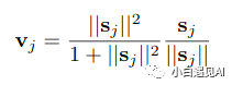
在探索算法之前,让我们先构造挤压函数(squash function)并保留以备将来使用。如果分母的总和为零,需要添加了一个小值的epsilon,以防止梯度爆炸。
epsilon = 1e-7def squash(self, s):s_norm = tf.norm(s, axis=-1, keepdims=True)return tf.square(s_norm)/(1 + tf.square(s_norm)) * s/(s_norm + epsilon)
在此步骤中,数字胶囊的输入是16D向量(u_hat),路由迭代次数(r = 3)。
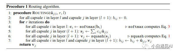
动态路由算法没有太多调整,并且代码几乎是本文中算法的直接实现。看看下面的代码片段。
b = tf.zeros((input_x.shape[0], 1152, 10, 1))for i in range(r):c = tf.nn.softmax(b, axis=-2) # c.shape: (None, 1152, 10, 1)s = tf.reduce_sum(tf.multiply(c, u_hat), axis=1, keepdims=True) # s.shape: (None, 1, 10, 16)v = squash(s) # v.shape: (None, 1, 10, 16)agreement = tf.squeeze(tf.matmul(tf.expand_dims(u_hat, axis=-1), tf.expand_dims(v, axis=-1), transpose_a=True), [4]) # agreement.shape: (None, 1152, 10, 1)# Before matmul following intermediate shapes are present, they are not assigned to a variable but just for understanding the code.# u_hat.shape (Intermediate shape) : (None, 1152, 10, 16, 1)# v.shape (Intermediate shape): (None, 1, 10, 16, 1)# Since the first parameter of matmul is to be transposed its shape becomes:(None, 1152, 10, 1, 16)# Now matmul is performed in the last two dimensions, and others are broadcasted# Before squeezing we have an intermediate shape of (None, 1152, 10, 1, 1)b += agreement
需要注意以下问题:
1.该c表示的概率分布u_hat值和在所述主胶囊层中的特定胶囊时,它概括为1。简单地说,u_hat的值根据其在路由算法训练变量c的数字胶囊中均有分布。
2.所述ΣcijUj|i是输入到数字胶囊低层向量的所有加权求和。由于存在1152个较低级别的向量,因此reduce_sum函数将应用到该维度。设置keep_dims=True,只会使进一步的计算更加容易。
3.挤压函数非线性将应用于Digit Capsule的16D向量,以将值归一化。
4.下一步是一个很巧妙的应用,在该应用中,将计算数字囊层的输入和输出之间的点积。这种点积决定了低级和高级级胶囊之间的“协议”。
重复上述循环3次,然后将由此获得的v值用于重建网络。
重建网络
重建网络是一种可从Digit Capsule Layers的特征再生图像的正则化器。在反向传播时,它会影响整个网络,因此使功能既适合预测又适合再生。在训练期间,模型使用输入图像的实际标签将数字上限的值屏蔽为零(与标签相对应的数字除外)(如下图所示)。
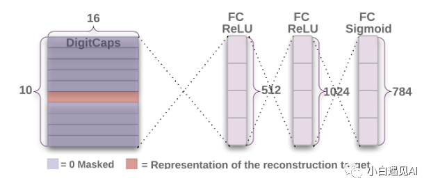
来自上述网络的张量的形状为(None,1,10,16),我们沿着Digit Caps图层的16D矢量广播和标记,并应用掩膜。
注意:一个热编码标签用于掩膜。
y = tf.expand_dims(y, axis=-1) # y.shape: (None, 10, 1)y = tf.expand_dims(y, axis=1) # y.shape: (None, 1, 10, 1)mask = tf.cast(y, dtype=tf.float32) # mask.shape: (None, 1, 10, 1)v_masked = tf.multiply(mask, v) # v_masked.shape: (None, 1, 10, 16
此v_masked被再发送到网络重建并且被用于整个图像的再生。重建网络只是下面要点中显示的3个密集层。
dense_1 = tf.keras.layers.Dense(units = 512, activation='relu')dense_2 = tf.keras.layers.Dense(units = 1024, activation='relu')dense_3 = tf.keras.layers.Dense(units = 784, activation='sigmoid', dtype='float32')v_ = tf.reshape(v_masked, [-1, 10 * 16]) # v_.shape: (None, 160)reconstructed_image = dense_1(v_) # reconstructed_image.shape: (None, 512)reconstructed_image = dense_2(reconstructed_image) # reconstructed_image.shape: (None, 1024)reconstructed_image = dense_3(reconstructed_image) # reconstructed_image.shape: (None, 784)
我们将上述相同代码转换为继承自的CapsuleNetwork类tf.keras.Model。也可以直接在自定义训练循环中使用该课程并进行预测。
class CapsuleNetwork(tf.keras.Model):def __init__(self, no_of_conv_kernels, no_of_primary_capsules, primary_capsule_vector, no_of_secondary_capsules, secondary_capsule_vector, r):super(CapsuleNetwork, self).__init__()self.no_of_conv_kernels = no_of_conv_kernelsself.no_of_primary_capsules = no_of_primary_capsulesself.primary_capsule_vector = primary_capsule_vectorself.no_of_secondary_capsules = no_of_secondary_capsulesself.secondary_capsule_vector = secondary_capsule_vectorself.r = rwith tf.name_scope("Variables") as scope:self.convolution = tf.keras.layers.Conv2D(self.no_of_conv_kernels, [9,9], strides=[1,1], name='ConvolutionLayer', activation='relu')self.primary_capsule = tf.keras.layers.Conv2D(self.no_of_primary_capsules * self.primary_capsule_vector, [9,9], strides=[2,2], name="PrimaryCapsule")self.w = tf.Variable(tf.random_normal_initializer()(shape=[1, 1152, self.no_of_secondary_capsules, self.secondary_capsule_vector, self.primary_capsule_vector]), dtype=tf.float32, name="PoseEstimation", trainable=True)self.dense_1 = tf.keras.layers.Dense(units = 512, activation='relu')self.dense_2 = tf.keras.layers.Dense(units = 1024, activation='relu')self.dense_3 = tf.keras.layers.Dense(units = 784, activation='sigmoid', dtype='float32')def build(self, input_shape):passdef squash(self, s):with tf.name_scope("SquashFunction") as scope:s_norm = tf.norm(s, axis=-1, keepdims=True)return tf.square(s_norm)/(1 + tf.square(s_norm)) * s/(s_norm + epsilon)@tf.functiondef call(self, inputs):input_x, y = inputs# input_x.shape: (None, 28, 28, 1)# y.shape: (None, 10)x = self.convolution(input_x) # x.shape: (None, 20, 20, 256)x = self.primary_capsule(x) # x.shape: (None, 6, 6, 256)with tf.name_scope("CapsuleFormation") as scope:u = tf.reshape(x, (-1, self.no_of_primary_capsules * x.shape[1] * x.shape[2], 8)) # u.shape: (None, 1152, 8)u = tf.expand_dims(u, axis=-2) # u.shape: (None, 1152, 1, 8)u = tf.expand_dims(u, axis=-1) # u.shape: (None, 1152, 1, 8, 1)u_hat = tf.matmul(self.w, u) # u_hat.shape: (None, 1152, 10, 16, 1)u_hat = tf.squeeze(u_hat, [4]) # u_hat.shape: (None, 1152, 10, 16)with tf.name_scope("DynamicRouting") as scope:b = tf.zeros((input_x.shape[0], 1152, self.no_of_secondary_capsules, 1)) # b.shape: (None, 1152, 10, 1)for i in range(self.r): # self.r = 3c = tf.nn.softmax(b, axis=-2) # c.shape: (None, 1152, 10, 1)s = tf.reduce_sum(tf.multiply(c, u_hat), axis=1, keepdims=True) # s.shape: (None, 1, 10, 16)v = self.squash(s) # v.shape: (None, 1, 10, 16)agreement = tf.squeeze(tf.matmul(tf.expand_dims(u_hat, axis=-1), tf.expand_dims(v, axis=-1), transpose_a=True), [4]) # agreement.shape: (None, 1152, 10, 1)# Before matmul following intermediate shapes are present, they are not assigned to a variable but just for understanding the code.# u_hat.shape (Intermediate shape) : (None, 1152, 10, 16, 1)# v.shape (Intermediate shape): (None, 1, 10, 16, 1)# Since the first parameter of matmul is to be transposed its shape becomes:(None, 1152, 10, 1, 16)# Now matmul is performed in the last two dimensions, and others are broadcasted# Before squeezing we have an intermediate shape of (None, 1152, 10, 1, 1)b += agreementwith tf.name_scope("Masking") as scope:y = tf.expand_dims(y, axis=-1) # y.shape: (None, 10, 1)y = tf.expand_dims(y, axis=1) # y.shape: (None, 1, 10, 1)mask = tf.cast(y, dtype=tf.float32) # mask.shape: (None, 1, 10, 1)v_masked = tf.multiply(mask, v) # v_masked.shape: (None, 1, 10, 16)with tf.name_scope("Reconstruction") as scope:v_ = tf.reshape(v_masked, [-1, self.no_of_secondary_capsules * self.secondary_capsule_vector]) # v_.shape: (None, 160)reconstructed_image = self.dense_1(v_) # reconstructed_image.shape: (None, 512)reconstructed_image = self.dense_2(reconstructed_image) # reconstructed_image.shape: (None, 1024)reconstructed_image = self.dense_3(reconstructed_image) # reconstructed_image.shape: (None, 784)return v, reconstructed_image@tf.functiondef predict_capsule_output(self, inputs):x = self.convolution(inputs) # x.shape: (None, 20, 20, 256)x = self.primary_capsule(x) # x.shape: (None, 6, 6, 256)with tf.name_scope("CapsuleFormation") as scope:u = tf.reshape(x, (-1, self.no_of_primary_capsules * x.shape[1] * x.shape[2], 8)) # u.shape: (None, 1152, 8)u = tf.expand_dims(u, axis=-2) # u.shape: (None, 1152, 1, 8)u = tf.expand_dims(u, axis=-1) # u.shape: (None, 1152, 1, 8, 1)u_hat = tf.matmul(self.w, u) # u_hat.shape: (None, 1152, 10, 16, 1)u_hat = tf.squeeze(u_hat, [4]) # u_hat.shape: (None, 1152, 10, 16)with tf.name_scope("DynamicRouting") as scope:b = tf.zeros((inputs.shape[0], 1152, self.no_of_secondary_capsules, 1)) # b.shape: (None, 1152, 10, 1)for i in range(self.r): # self.r = 3c = tf.nn.softmax(b, axis=-2) # c.shape: (None, 1152, 10, 1)s = tf.reduce_sum(tf.multiply(c, u_hat), axis=1, keepdims=True) # s.shape: (None, 1, 10, 16)v = self.squash(s) # v.shape: (None, 1, 10, 16)agreement = tf.squeeze(tf.matmul(tf.expand_dims(u_hat, axis=-1), tf.expand_dims(v, axis=-1), transpose_a=True), [4]) # agreement.shape: (None, 1152, 10, 1)# Before matmul following intermediate shapes are present, they are not assigned to a variable but just for understanding the code.# u_hat.shape (Intermediate shape) : (None, 1152, 10, 16, 1)# v.shape (Intermediate shape): (None, 1, 10, 16, 1)# Since the first parameter of matmul is to be transposed its shape becomes:(None, 1152, 10, 1, 16)# Now matmul is performed in the last two dimensions, and others are broadcasted# Before squeezing we have an intermediate shape of (None, 1152, 10, 1, 1)b += agreementreturn v@tf.functiondef regenerate_image(self, inputs):with tf.name_scope("Reconstruction") as scope:v_ = tf.reshape(inputs, [-1, self.no_of_secondary_capsules * self.secondary_capsule_vector]) # v_.shape: (None, 160)reconstructed_image = self.dense_1(v_) # reconstructed_image.shape: (None, 512)reconstructed_image = self.dense_2(reconstructed_image) # reconstructed_image.shape: (None, 1024)reconstructed_image = self.dense_3(reconstructed_image) # reconstructed_image.shape: (None, 784)return reconstructed_image
这里添加了两个不同的函数predict_capsule_output(),regenerate_image()它们分别预测数字Caps向量并分别重新生成图像。第一个功能将有助于预测测试期间的数字,第二个功能将有助于从给定的一组输入特征中重新生成图像。(将在可视化中使用)。
epsilon = 1e-7m_plus = 0.9m_minus = 0.1lambda_ = 0.5alpha = 0.0005epochs = 100params = {"no_of_conv_kernels": 256,"no_of_primary_capsules": 32,"no_of_secondary_capsules": 10,"primary_capsule_vector": 8,"secondary_capsule_vector": 16,"r":3,}model = CapsuleNetwork(**params)
因此,剩下的最后一件事就是损失函数。本文使用边际损失进行分类,并使用平方差进行权重为0.0005的重建来重建损失。参数m+,m-,λ在上面的要点中描述,而损失函数在下面的要点中描述。

def loss_function(v, reconstructed_image, y, y_image):prediction = safe_norm(v)prediction = tf.reshape(prediction, [-1, no_of_secondary_capsules])left_margin = tf.square(tf.maximum(0.0, m_plus - prediction))right_margin = tf.square(tf.maximum(0.0, prediction - m_minus))l = tf.add(y * left_margin, lambda_ * (1.0 - y) * right_margin)margin_loss = tf.reduce_mean(tf.reduce_sum(l, axis=-1))y_image_flat = tf.reshape(y_image, [-1, 784])reconstruction_loss = tf.reduce_mean(tf.square(y_image_flat - reconstructed_image))loss = tf.add(margin_loss, alpha * reconstruction_loss)return loss
v是未进行掩膜的数字胶囊矢量,y是标签的one_hot_encoded载体,y_image是实际发送图像输入到模型。安全规范函数(safe norm function)只是一个类似于TensorFlow规范函数的函数,但包含一个epsilon以避免该值变为精确的0。
def safe_norm(v, axis=-1):v_ = tf.reduce_sum(tf.square(v), axis = axis, keepdims=True)return tf.sqrt(v_ + epsilon)
让我们检查模型的摘要。
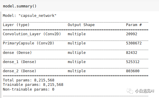
到这里我们已经完成了模型架构。该模型具有8215568个参数,与论文说的一样,他们说重构的模型具有8.2M个参数。但是,此博客具有8238608参数。差异的原因是TensorFlow仅考虑tf.Variable可训练参数中的资源。如果我们认为1152 * 10 b和1152 * 10 c是可训练的,那么我们得到相同的数字。
8215568 + 11520 + 11520 = 8238608
其他详细信息
我们将使用tf.GradientTape来查找渐变,并使用Adam优化器。
def train(x,y):y_one_hot = tf.one_hot(y, depth=10)with tf.GradientTape() as tape:v, reconstructed_image = model([x, y_one_hot])loss = loss_function(v, reconstructed_image, y_one_hot, x)grad = tape.gradient(loss, model.trainable_variables)optimizer.apply_gradients(zip(grad, model.trainable_variables))return loss
由于我们已使用来将类别细分为类别tf.keras.Model,因此我们可以简单地调用model.trainable_variables并应用渐变。
def predict(model, x):pred = safe_norm(model.predict_capsule_output(x))pred = tf.squeeze(pred, [1])return np.argmax(pred, axis=1)[:,0]
这里做了一个自定义的预测函数,它将输入图像以及模型作为参数。发送模型作为参数的目的是,可以将检查点模型稍后用于预测。
结果和特征可视化
该模型的训练精度为99%,测试精度为98%。但是,在某些检查点中,准确度为98.4%,而在其他一些检查点中为97.7%。
在下面的要点中,是index_指测试集中的特定样品编号,是index指样品所y_test[index_] 代表的实际编号。
print(predict(model, tf.expand_dims(X_test[index_], axis=0)), y_test[index_])features = model.predict_capsule_output(tf.expand_dims(X_test[index_], axis=0))temp_features = features.numpy()temp_ = temp_features.copy()temp_features[:,:,:,:] = 0temp_features[:,:,index,:] = temp_[:,:,index,:]recon = model.regenerate_image(temp_features)recon = tf.reshape(recon, (28,28))plt.subplot(1,2,1)plt.imshow(recon, cmap='gray')plt.subplot(1,2,2)plt.imshow(X_test[index_,:,:,0], cmap='gray')
下面的代码调整每个功能,并在[-0.25,0.25]范围内以0.05为增量进行调整。在每个点上,都会生成图像并将其存储在数组中。因此,我们可以看到每个特征如何促进图像重建。
col = np.zeros((28,308))for i in range(16):feature_ = temp_features.copy()feature_[:,:,index, i] += -0.25row = np.zeros((28,28))for j in range(10):feature_[:,:,index, i] += 0.05row = np.hstack([row, tf.reshape(model.regenerate_image(tf.convert_to_tensor(feature_)), (28,28)).numpy()])col = np.vstack([col, row])plt.figure(figsize=(30,20))plt.imshow(col[28:, 28:], cmap='gray')
请参见下图的一些重建示例。我们可以看到,某些功能控制着亮度,旋转角度,厚度,偏斜度等。

结论
在本文中,我们试图重现结果并可视化本文中描述的功能。训练精度为99%,测试精度几乎为98%,这确实很棒。虽然,该模型需要花费很多时间进行训练,但是功能非常直观。