教你使用TensorFlow2对阿拉伯语手写字符数据集进行识别-技术圈

「@Author：Runsen」

在本教程中，我们将使用 TensorFlow (Keras API) 实现一个用于多分类任务的深度学习模型，该任务需要对阿拉伯语手写字符数据集进行识别。

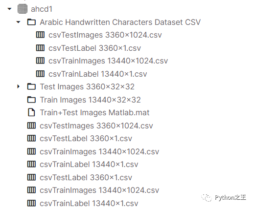
数据集下载地址：https://www.kaggle.com/mloey1/ahcd1

数据集介绍

该数据集由 60 名参与者书写的16,800 个字符组成，年龄范围在 19 至 40 岁之间，90% 的参与者是右手。

每个参与者在两种形式上写下每个字符（从“alef”到“yeh”）十次，如图 7（a）和 7（b）所示。表格以 300 dpi 的分辨率扫描。使用 Matlab 2016a 自动分割每个块以确定每个块的坐标。该数据库分为两组：训练集（每类 13,440 个字符到 480 个图像）和测试集（每类 3,360 个字符到 120 个图像）。数据标签为1到28个类别。在这里，所有数据集都是CSV文件，表示图像像素值及其相应标签，并没有提供对应的图片数据。

导入模块

import numpy as np
import pandas as pd
#允许对dataframe使用display（）
from IPython.display import display
# 导入读取和处理图像所需的库
import csv
from PIL import Image
from scipy.ndimage import rotate

读取数据

# 训练数据images
letters_training_images_file_path = "../input/ahcd1/csvTrainImages 13440x1024.csv"
# 训练数据labels
letters_training_labels_file_path = "../input/ahcd1/csvTrainLabel 13440x1.csv"
# 测试数据images和labels
letters_testing_images_file_path = "../input/ahcd1/csvTestImages 3360x1024.csv"
letters_testing_labels_file_path = "../input/ahcd1/csvTestLabel 3360x1.csv"

# 加载数据
training_letters_images = pd.read_csv(letters_training_images_file_path, header=None)
training_letters_labels = pd.read_csv(letters_training_labels_file_path, header=None)
testing_letters_images = pd.read_csv(letters_testing_images_file_path, header=None)
testing_letters_labels = pd.read_csv(letters_testing_labels_file_path, header=None)

print("%d个32x32像素的训练阿拉伯字母图像。" %training_letters_images.shape[0])
print("%d个32x32像素的测试阿拉伯字母图像。" %testing_letters_images.shape[0])
training_letters_images.head()

13440个32x32像素的训练阿拉伯字母图像。3360个32x32像素的测试阿拉伯字母图像。

查看训练数据的head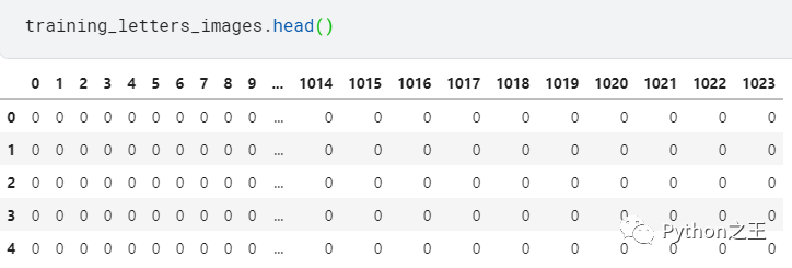

np.unique(training_letters_labels)
array([ 1,  2,  3,  4,  5,  6,  7,  8,  9, 10, 11, 12, 13, 14, 15, 16, 17,18, 19, 20, 21, 22, 23, 24, 25, 26, 27, 28], dtype=int32)

下面需要将csv值转换为图像，我们希望展示对应图像的像素值图像。

def convert_values_to_image(image_values, display=False):
    image_array = np.asarray(image_values)
    image_array = image_array.reshape(32,32).astype('uint8')
    # 原始数据集被反射，因此我们将使用np.flip翻转它，然后通过rotate旋转，以获得更好的图像。
    image_array = np.flip(image_array, 0)
    image_array = rotate(image_array, -90)
    new_image = Image.fromarray(image_array)
    if display == True:
        new_image.show()
    return new_image
convert_values_to_image(training_letters_images.loc[0], True)

这是一个字母f。

下面，我们将进行数据预处理，主要进行图像标准化，我们通过将图像中的每个像素除以255来重新缩放图像，标准化到[0，1]

training_letters_images_scaled = training_letters_images.values.astype('float32')/255
training_letters_labels = training_letters_labels.values.astype('int32')
testing_letters_images_scaled = testing_letters_images.values.astype('float32')/255
testing_letters_labels = testing_letters_labels.values.astype('int32')
print("Training images of letters after scaling")
print(training_letters_images_scaled.shape)
training_letters_images_scaled[0:5]

输出如下

Training images of letters after scaling
(13440, 1024)

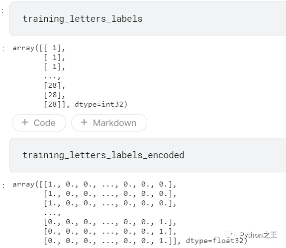
从标签csv文件我们可以看到，这是一个多类分类问题。下一步需要进行分类标签编码，建议将类别向量转换为矩阵类型。

输出形式如下：将1到28，变成0到27类别。从“alef”到“yeh”的字母有0到27的分类号。to_categorical就是将类别向量转换为二进制（只有0和1）的矩阵类型表示

在这里，我们将使用keras的一个热编码对这些类别值进行编码。

一个热编码将整数转换为二进制矩阵，其中数组仅包含一个“1”，其余元素为“0”。

from keras.utils import to_categorical

# one hot encoding
number_of_classes = 28

training_letters_labels_encoded = to_categorical(training_letters_labels-1, num_classes=number_of_classes)
testing_letters_labels_encoded = to_categorical(testing_letters_labels-1, num_classes=number_of_classes)

# (13440, 1024)

下面将输入图像重塑为32x32x1，因为当使用TensorFlow作为后端时，Keras CNN需要一个4D数组作为输入，并带有形状（nb_samples、行、列、通道）

其中 nb_samples对应于图像（或样本）的总数，而行、列和通道分别对应于每个图像的行、列和通道的数量。

# reshape input letter images to 32x32x1
training_letters_images_scaled = training_letters_images_scaled.reshape([-1, 32, 32, 1])
testing_letters_images_scaled = testing_letters_images_scaled.reshape([-1, 32, 32, 1])

print(training_letters_images_scaled.shape, training_letters_labels_encoded.shape, testing_letters_images_scaled.shape, testing_letters_labels_encoded.shape)
# (13440, 32, 32, 1) (13440, 28) (3360, 32, 32, 1) (3360, 28)

因此，我们将把输入图像重塑成4D张量形状（nb_samples，32，32，1），因为我们图像是32x32像素的灰度图像。

#将输入字母图像重塑为32x32x1
training_letters_images_scaled = training_letters_images_scaled.reshape([-1, 32, 32, 1])
testing_letters_images_scaled = testing_letters_images_scaled.reshape([-1, 32, 32, 1])

print(training_letters_images_scaled.shape, training_letters_labels_encoded.shape, testing_letters_images_scaled.shape, testing_letters_labels_encoded.shape)

设计模型结构

from keras.models import Sequential
from keras.layers import Conv2D, MaxPooling2D, GlobalAveragePooling2D, BatchNormalization, Dropout, Dense

def create_model(optimizer='adam', kernel_initializer='he_normal', activation='relu'):
    # create model
    model = Sequential()
    model.add(Conv2D(filters=16, kernel_size=3, padding='same', input_shape=(32, 32, 1), kernel_initializer=kernel_initializer, activation=activation))
    model.add(BatchNormalization())
    model.add(MaxPooling2D(pool_size=2))
    model.add(Dropout(0.2))

    model.add(Conv2D(filters=32, kernel_size=3, padding='same', kernel_initializer=kernel_initializer, activation=activation))
    model.add(BatchNormalization())
    model.add(MaxPooling2D(pool_size=2))
    model.add(Dropout(0.2))

    model.add(Conv2D(filters=64, kernel_size=3, padding='same', kernel_initializer=kernel_initializer, activation=activation))
    model.add(BatchNormalization())
    model.add(MaxPooling2D(pool_size=2))
    model.add(Dropout(0.2))

    model.add(Conv2D(filters=128, kernel_size=3, padding='same', kernel_initializer=kernel_initializer, activation=activation))
    model.add(BatchNormalization())
    model.add(MaxPooling2D(pool_size=2))
    model.add(Dropout(0.2))
    model.add(GlobalAveragePooling2D())

    #Fully connected final layer
    model.add(Dense(28, activation='softmax'))

    # Compile model
    model.compile(loss='categorical_crossentropy', metrics=['accuracy'], optimizer=optimizer)
    return model

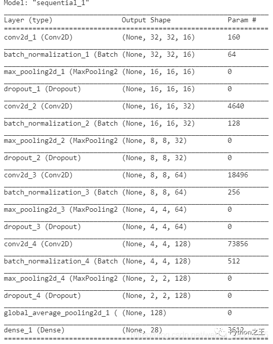
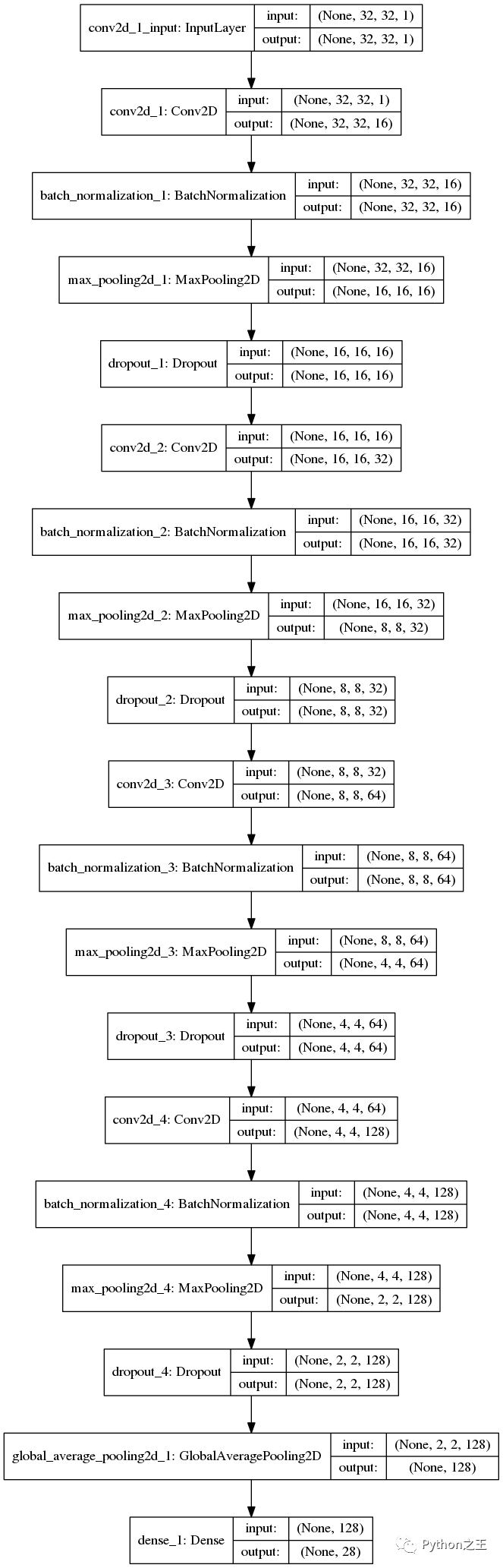
「模型结构」

第一隐藏层是卷积层。该层有16个特征图，大小为3×3和一个激活函数，它是relu。这是输入层，需要具有上述结构的图像。
第二层是批量标准化层，它解决了特征分布在训练和测试数据中的变化，BN层添加在激活函数前，对输入激活函数的输入进行归一化。这样解决了输入数据发生偏移和增大的影响。
第三层是MaxPooling层。最大池层用于对输入进行下采样，使模型能够对特征进行假设，从而减少过拟合。它还减少了参数的学习次数，减少了训练时间。
下一层是使用dropout的正则化层。它被配置为随机排除层中20%的神经元，以减少过度拟合。
另一个隐藏层包含32个要素，大小为3×3和relu激活功能，从图像中捕捉更多特征。
其他隐藏层包含64和128个要素，大小为3×3和一个relu激活功能，
重复三次卷积层、MaxPooling、批处理规范化、正则化和* GlobalAveragePooling2D层。
最后一层是具有（输出类数）的输出层，它使用softmax激活函数，因为我们有多个类。每个神经元将给出该类的概率。
使用分类交叉熵作为损失函数，因为它是一个多类分类问题。使用精确度作为衡量标准来提高神经网络的性能。

model = create_model(optimizer='Adam', kernel_initializer='uniform', activation='relu')
model.summary()

「Keras支持在Keras.utils.vis_utils模块中绘制模型，该模块提供了使用graphviz绘制Keras模型的实用函数」


import pydot
from keras.utils import plot_model

plot_model(model, to_file="model.png", show_shapes=True)
from IPython.display import Image as IPythonImage
display(IPythonImage('model.png'))

训练模型，使用batch_size=20来训练模型，对模型进行15个epochs阶段的训练。


from keras.callbacks import ModelCheckpoint  

# 使用检查点来保存稍后使用的模型权重。
checkpointer = ModelCheckpoint(filepath='weights.hdf5', verbose=1, save_best_only=True)
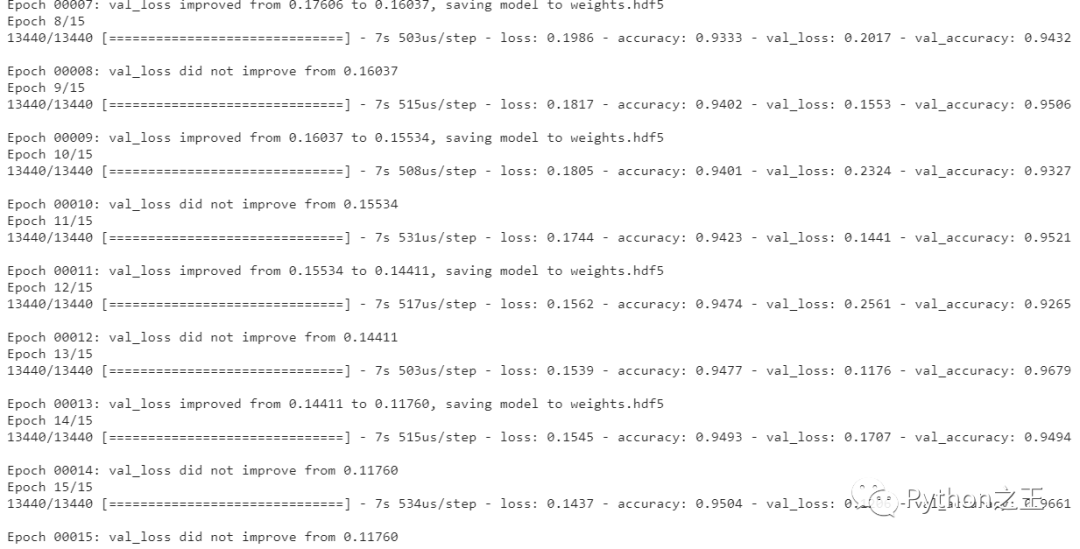
history = model.fit(training_letters_images_scaled, training_letters_labels_encoded,validation_data=(testing_letters_images_scaled,testing_letters_labels_encoded),epochs=15, batch_size=20, verbose=1, callbacks=[checkpointer])

训练结果如下所示：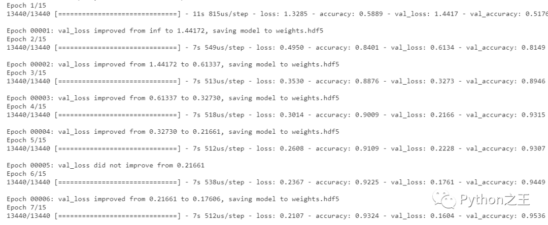

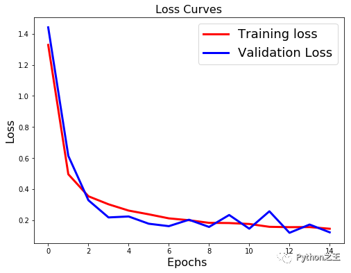
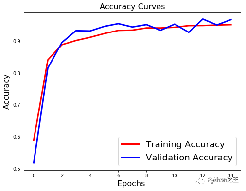
最后Epochs绘制损耗和精度曲线。


import matplotlib.pyplot as plt

def plot_loss_accuracy(history):
    # Loss 
    plt.figure(figsize=[8,6])
    plt.plot(history.history['loss'],'r',linewidth=3.0)
    plt.plot(history.history['val_loss'],'b',linewidth=3.0)
    plt.legend(['Training loss', 'Validation Loss'],fontsize=18)
    plt.xlabel('Epochs ',fontsize=16)
    plt.ylabel('Loss',fontsize=16)
    plt.title('Loss Curves',fontsize=16)

    # Accuracy 
    plt.figure(figsize=[8,6])
    plt.plot(history.history['accuracy'],'r',linewidth=3.0)
    plt.plot(history.history['val_accuracy'],'b',linewidth=3.0)
    plt.legend(['Training Accuracy', 'Validation Accuracy'],fontsize=18)
    plt.xlabel('Epochs ',fontsize=16)
    plt.ylabel('Accuracy',fontsize=16)
    plt.title('Accuracy Curves',fontsize=16) 

plot_loss_accuracy(history)

「加载具有最佳验证损失的模型」

# 加载具有最佳验证损失的模型
model.load_weights('weights.hdf5')
metrics = model.evaluate(testing_letters_images_scaled, testing_letters_labels_encoded, verbose=1)
print("Test Accuracy: {}".format(metrics[1]))
print("Test Loss: {}".format(metrics[0]))

输出如下：

3360/3360 [==============================] - 0s 87us/step
Test Accuracy: 0.9678571224212646
Test Loss: 0.11759862171020359

打印混淆矩阵。

from sklearn.metrics import classification_report

def get_predicted_classes(model, data, labels=None):
    image_predictions = model.predict(data)
    predicted_classes = np.argmax(image_predictions, axis=1)
    true_classes = np.argmax(labels, axis=1)
    return predicted_classes, true_classes, image_predictions

def get_classification_report(y_true, y_pred):
    print(classification_report(y_true, y_pred))


y_pred, y_true, image_predictions = get_predicted_classes(model, testing_letters_images_scaled, testing_letters_labels_encoded)
get_classification_report(y_true, y_pred)

输出如下：

              precision    recall  f1-score   support

           0       1.00      0.98      0.99       120
           1       1.00      0.98      0.99       120
           2       0.80      0.98      0.88       120
           3       0.98      0.88      0.93       120
           4       0.99      0.97      0.98       120
           5       0.92      0.99      0.96       120
           6       0.94      0.97      0.95       120
           7       0.94      0.95      0.95       120
           8       0.96      0.88      0.92       120
           9       0.90      1.00      0.94       120
          10       0.94      0.90      0.92       120
          11       0.98      1.00      0.99       120
          12       0.99      0.98      0.99       120
          13       0.96      0.97      0.97       120
          14       1.00      0.93      0.97       120
          15       0.94      0.99      0.97       120
          16       1.00      0.93      0.96       120
          17       0.97      0.97      0.97       120
          18       1.00      0.93      0.96       120
          19       0.92      0.95      0.93       120
          20       0.97      0.93      0.94       120
          21       0.99      0.96      0.97       120
          22       0.99      0.98      0.99       120
          23       0.98      0.99      0.99       120
          24       0.95      0.88      0.91       120
          25       0.94      0.98      0.96       120
          26       0.95      0.97      0.96       120
          27       0.98      0.99      0.99       120

    accuracy                           0.96      3360
   macro avg       0.96      0.96      0.96      3360
weighted avg       0.96      0.96      0.96      3360

最后绘制随机几个相关预测的图片

indices = np.random.randint(0, testing_letters_labels.shape[0], size=49)
y_pred = np.argmax(model.predict(training_letters_images_scaled), axis=1)

for i, idx in enumerate(indices):
    plt.subplot(7,7,i+1)
        
    image_array = training_letters_images_scaled[idx][:,:,0]
    image_array = np.flip(image_array, 0)
    image_array = rotate(image_array, -90)
       
    plt.imshow(image_array, cmap='gray')
    plt.title("Pred: {} - Label: {}".format(y_pred[idx], (training_letters_labels[idx] -1)))
    plt.xticks([])
    plt.yticks([])
plt.show()