UMAP 是怎么把 Hinton 的 t-SNE 淘汰掉的？

共 5724字，需浏览 12分钟

· 2020-12-17

1摘要

本文将尝试介绍 UMAP 背后的数学原理及代码实现，并对 t-SNE 与 UMAP 进行详细比较，以探究为什么 UMAP 算法能够更快、更准地抓住数据的全局结构。我们还将尝试使用 Python 从头实现 t-SNE 和 UMAP。由于这些算法经典并且非常实用，因此值得花些时间来研究一番。

.目录

tSNE 已挂，UMAP 万岁！
关于 tSNE 的工作原理的简要回顾
从头开始编程实现 tSNE 算法
tSNE 和 UMAP 之间的关键区别
为什么 tSNE 只保留局部结构？
为什么 UMAP 可以保留全局结构
从头开始编程实现 UMAP 算法
为什么 UMAP 跑起来比 tSNE 快

.t-SNE 已挂， UMAP 万岁！

如果你不知道 t-SNE 是什么？也不知道它是如何工作的？更没有阅读提出它的那篇革命性的论文 van der Maaten ＆ Hinton 在 2008 年发表的论文^[1] 的话，你可能不需要知道，因为 t-SNE 现在基本上已经挂掉了。尽管 t-SNE 总体上对单细胞基因组学和数据科学产生了巨大影响，但人们普遍认为 t-SNE 具有一些迟早必须解决的缺点。

到底是什么使我们对单细胞基因组学使用 t-SNE 感到不舒服呢？我们来简单总结下：

t-SNE 无法很好地适应对于数据样本量快速增加的情况。如果尝试使用 FIt-SNE 加快速度，将会导致极大的内存消耗，从而无法在计算机群集之外进行分析。
t-SNE 不会保留全局结构，这意味着只有在簇距离之内才有意义，而并不能保证簇间的相似性。

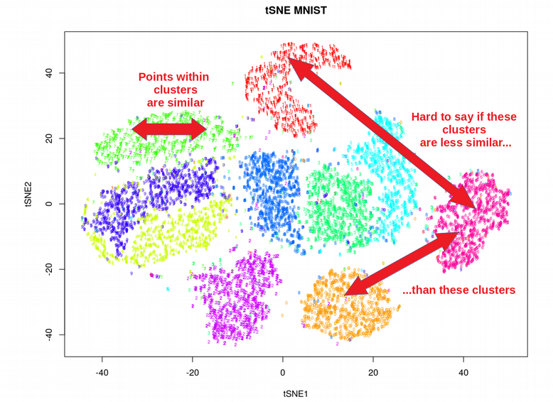
t-SNE 实际上只能嵌入 2 或 3 个维度，即仅用于可视化目的，因此很难将 t-SNE 当作一般的降维技术来使用，例如产生 10D 或 50D 的低维表示。注意，即使对于更现代的 FIt-SNE算法仍然存在此问题。
t-SNE 执行从高维空间到低维空间的非参数映射，这意味着它并不有效利用驱动数据聚类的那些特征。
t-SNE 不能直接处理高维数据，通常在使用 t-SNE 前会先执行 PCA 或 Autoencoder 对高维数据作降维预处理。
t-SNE 消耗过多内存，这在使用大的困惑度（一个超参数）时尤为明显，更现代的 FIt-SNE 算法也无法解决此问题。

.关于 t-SNE 工作原理的简短回顾

t-SNE 是一种相对比较简单的机器学习算法，可以用以下四个公式进行概括:

\begin{array}{lll} p_{j|i} = \dfrac{\exp \left ( - || x_i - x_j || ^2 \big / 2 \sigma_i^2 \right ) }{\sum_{k \neq i} \exp \left ( - || x_i - x_k || ^2 \big / 2 \sigma_i^2 \right )}, \\[2em] p_{ij} = \dfrac{p_{i|j} + p_{j|i}}{2N} \hspace{2em} (1) \end{array}

\rm{Perplexity} = \displaystyle 2^{\large -\sum_j p_{j|i} \log_2 p_{j|i}} \hspace{2em} (2)

q_{ij} = \frac{ \left ( 1 + || y_i - y_j || ^2 \right ) ^ {-1} }{\sum_{k \neq l} \left ( 1 + || y_k - y_l || ^2 \right ) ^ {-1} } \hspace{2em} (3)

\begin{array}{lll} &\text{KL}(P_i || Q_i) = \sum_i \sum_j p_{j|i} \log \dfrac {p_{j|i}} {q_{j|i}}, \\[1em]& \dfrac{\partial \text{KL}}{\partial y_i} = 4 \sum_j (p_{ij} - q_{ij}) (y_i - y_j) \left ( 1 + || y_i - y_j || ^2 \right ) ^ {-1} \hspace{2em} (4) \end{array}

等式 (1) 定义了高维空间中任何两点之间的距离的高斯概率，其满足对称条件。
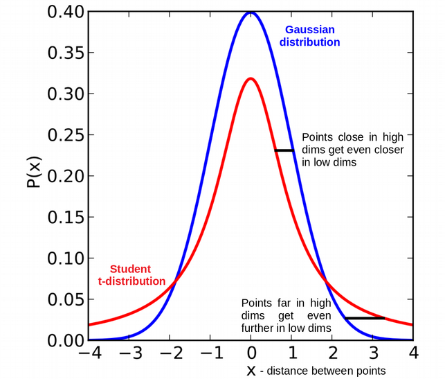
等式 (2) 引入了困惑度（Perplexity）的概念，它为确定每个样本的最优（高斯分布中的参数，即标准差）提供了依据。
等式 (3) 为低维嵌入中的点对之间的距离使用了学生 t-分布。当嵌入到低维度时，t-分布的长尾效应将可以克服低维嵌入中的拥挤问题。
等式 (4) 提供了将高维分布投影到低维分布上的 Kullback-Leibler 散度损失函数，以及推导了梯度下降法中使用到的梯度的解析形式。

由于 t-SNE 算法原理相对简单，因此让我们尝试用 Python 从头来实现它吧。通常，我们需要导入必要的 Python 库，这里我们将主要使用 numpy。

.从头开始编程实现 t-SNE

作为测试数据集，我们将使用癌相关成纤维细胞（CAF）^[2] scRNAseq 数据。我们从导入 Python 库开始（主要使用 numpy 和 scikit-learn），先看一下数据矩阵并检查数据集的维度。请注意，这里的行是细胞，列是基因，最后一列包含聚类结果的编码，即所有细胞都属于 #1、#2、#3 或 #4 四个聚类。

import numpy as np
import pandas as pd
import matplotlib.pyplot as plt
from sklearn.metrics.pairwise import euclidean_distances

path = './'
expr = pd.read_csv(path + 'CAFs.txt', sep='\t')
print(expr.iloc[0:4,0:4])

X_train = expr.values[:,0:(expr.shape[1]-1)]
X_train = np.log(X_train + 1)
n = X_train.shape[0]
print("\nThis data set contains " + str(n) + " samples")

y_train = expr.values[:,expr.shape[1]-1]
print("\nDimensions of the  data set: ")
print(X_train.shape, y_train.shape)

                1110020A21Rik  1110046J04Rik  1190002F15Rik  1500015A07Rik
SS2_15_0048_A3            0.0            0.0            0.0            0.0
SS2_15_0048_A6            0.0            0.0            0.0            0.0
SS2_15_0048_A5            0.0            0.0            0.0            0.0
SS2_15_0048_A4            0.0            0.0            0.0            0.0

This data set contains 716 samples

Dimensions of the  data set: 
(716, 557) (716,)

y_train[::10]

array([1., 2., 1., 1., 1., 1., 2., 1., 2., 1., 2., 2., 1., 4., 2., 4., 3.,
       1., 1., 1., 2., 1., 2., 2., 2., 4., 1., 1., 1., 1., 1., 1., 1., 1.,
       1., 2., 1., 1., 4., 4., 1., 1., 4., 2., 2., 1., 1., 1., 1., 1., 1.,
       1., 2., 1., 1., 1., 3., 3., 1., 4., 2., 1., 1., 1., 1., 4., 1., 2.,
       1., 1., 2., 1.])

先计算一个重要的全局变量，点对距离矩阵，记录了初始高维数据集 scRNAseq 中的数据两两之间的欧氏距离的平方，以后代码中将大量使用该矩阵。

dist = np.square(euclidean_distances(X_train, X_train))
dist[0:4, 0:4]

array([[   0.        ,  914.95016311, 1477.46836099, 3036.91172176],
       [ 914.95016311,    0.        , 1307.39294642, 2960.41559961],
       [1477.46836099, 1307.39294642,    0.        , 2678.34442573],
       [3036.91172176, 2960.41559961, 2678.34442573,    0.        ]])

接下来，我们将根据等式 (1) 使用上面的距离矩阵来计算高维空间中的概率矩阵。有了该矩阵，我们可以很容易计算熵和困惑度。请注意函数的参数 sigma。这意味着概率矩阵是的函数，而参数将在后面使用二分查找确定，即给定困惑度后计算最优的。

def prob_high_dim(sigma, dist_row):
    """
    For each row of Euclidean distance matrix (dist_row) compute
    probability in high dimensions (1D array)
    """
    exp_distance = np.exp(-dist[dist_row] / (2sigma*2))
    exp_distance[dist_row] = 0
    prob_not_symmetr = exp_distance / np.sum(exp_distance)
    # prob_symmetr = (prob_not_symmetr + prob_not_symmetr.T) / (2*n_samples)
    return prob_not_symmetr

def perplexity(prob):
    """
    Compute perplexity (scalar) for each 1D array of high-dimensional probability
    """
    return np.power(2, -np.sum([p*np.log2(p) for p in prob if p!=0]))

这里的一个技巧是，为了方便起见，为第 i 个数据，即距离矩阵的第 i 行（或列），计算一维概率数组（从第 i 个数据到数据集中的所有其它数据）。之所以这样做，是因为式 (1) 中的指数，即我们将使用二分查找为数据集中的每个数据计算合适的。
接者，对于第 i 个数据，给定一维高维概率的数组，我们可以对数组中的元素求和，并根据式 (2) 的定义计算出困惑度。因此，我们有一个函数，它为第 i 个数据的生成困惑度值（一个标量）。
现在我们可以设定困惑度值（即期望的困惑度，也称为超参数），并将此函数放入下面的二分查找过程中，以便计算 :

困惑度由计算而来，但后者不知道啊，而每个数据点都不一样。那么在给定困惑度的前提下，用二分查找法搜索合适的值。困惑度量化了点周围的秩序，相同秩序下稠密不同的区域对应不同的。

def sigma_binary_search(perp_of_sigma, fixed_perplexity):
    """
    Solve equation perp_of_sigma(sigma) = fixed_perplexity 
    with respect to sigma by the binary search algorithm
    """
    sigma_lower_limit = 0
    sigma_upper_limit = 1000
    for i in range(20):
        approx_sigma = (sigma_lower_limit + sigma_upper_limit) / 2
        if perp_of_sigma(approx_sigma) < fixed_perplexity:
            sigma_lower_limit = approx_sigma
        else:
            sigma_upper_limit = approx_sigma
        if np.abs(fixed_perplexity - perp_of_sigma(approx_sigma)) <= 1e-5:
            break
    return approx_sigma

最后，我们可以定义的一个 lambda 函数来计算困惑度，将所需的困惑度固定，例如 30，并对每个数据点使用二分查找搜索合适的。对于数据点，得到，并将其代回公式 (1) 计算高维空间中点对的欧几里得距离的概率矩阵。从技术上讲，每个数据点对应一个一维概率数组；那么计算每个数据点的，我们将得到 n 个一维概率数组，这些数组共同构成了高维概率矩阵。

PERPLEXITY = 30
prob = np.zeros((n,n))
sigma_array = []

for dist_row in range(n):

    func = lambda sigma: perplexity(prob_high_dim(sigma, dist_row))
    binary_search_result = sigma_binary_search(func, PERPLEXITY)
    
    prob[dist_row] = prob_high_dim(binary_search_result, dist_row)
    sigma_array.append(binary_search_result)
    
    if (dist_row + 1) % 100 == 0:
        print("Sigma binary search finished {0} of {1} cells".format(dist_row + 1, n))

print("\nMean sigma = " + str(np.mean(sigma_array)))

Sigma binary search finished 100 of 716 cells
Sigma binary search finished 200 of 716 cells
Sigma binary search finished 300 of 716 cells
Sigma binary search finished 400 of 716 cells
Sigma binary search finished 500 of 716 cells
Sigma binary search finished 600 of 716 cells
Sigma binary search finished 700 of 716 cells

Mean sigma = 6.374859943070225

np.array(sigma_array)[0:20]

array([4.8456192 , 5.51700592, 5.00965118, 7.05623627, 6.4496994 ,
       8.22734833, 7.05432892, 5.62000275, 6.75868988, 5.3396225 ,
       7.68375397, 7.06005096, 5.95569611, 5.46550751, 4.69493866,
       5.47504425, 7.12680817, 6.15596771, 7.15732574, 5.60474396])

prob[0:4, 0:4]

array([[0.00000000e+00, 1.56103054e-02, 9.79824059e-08, 3.70810924e-22],
       [3.07204951e-03, 0.00000000e+00, 4.87134781e-06, 7.84507211e-18],
       [3.14890611e-05, 9.32673319e-04, 0.00000000e+00, 1.28124979e-15],
       [2.09788702e-09, 4.52270838e-09, 7.68375118e-08, 0.00000000e+00]])

最后，我们来实现公式 (1) 中的对称条件。

P = prob + np.transpose(prob)
# P = (prob + np.transpose(prob)) / (2*n)
# P = P / np.sum(P)

好了，到此我们完成了公式 (1) 和 (2)。

代码主要部分完成了，实现公式 (3) 中的低维嵌入相对简单。注意，计算低维概率矩阵的公式 (3) 以低维嵌入的坐标 Y 作为参数。这意味着 Y 坐标将在后面通过 KL-散度来优化求解。

def prob_low_dim(Y):
    """
    Compute matrix of probabilities q_ij in low-dimensional space
    """
    inv_distances = np.power(1 + np.square(euclidean_distances(Y, Y)), -1)
    np.fill_diagonal(inv_distances, 0.)
    return inv_distances / np.sum(inv_distances, axis = 1, keepdims = True)

实际上，我们不需要实现公式 (4) 中的 KL-散度的定义。在代码中，我们只需要计算 KL-散度关于低维嵌入坐标 Y 的梯度。但是，仍然可以在每次梯度下降迭代中计算一下 KL-散度，用以输出查看，确保在优化过程中它确实在减小。

def KL(P, Y):
    """
    Compute KL-divergence from matrix of high-dimensional probabilities 
    and coordinates of low-dimensional embeddings
    """
    Q = prob_low_dim(Y)
    return P  np.log(P + 0.01) - P  np.log(Q + 0.01)

计算公式 (4) 中的 KL-散度的梯度时需要一点技巧，这里使用了Liam Schoneveld 博客^[3]中的方法。

def KL_gradient(P, Y):
    """
    Compute gradient of KL-divergence
    """
    Q = prob_low_dim(Y)
    y_diff = np.expand_dims(Y, 1) - np.expand_dims(Y, 0)
    inv_dist = np.power(1 + np.square(euclidean_distances(Y, Y)), -1)
    return 4np.sum(np.expand_dims(P - Q, 2)  y_diff * np.expand_dims(inv_dist, 2), axis = 1)

到此，一切准备就绪，可以运行梯度下降大法进行优化。我们将使用正态分布初始化低维嵌入的坐标 Y，并通过梯度下降法更新 Y。在优化过程中将对 KL-散度进行监控。

N_LOW_DIMS = 2
LEARNING_RATE = 0.6
MAX_ITER = 200

np.random.seed(12345)
y = np.random.normal(loc = 0, scale = 1, size = (n, N_LOW_DIMS))
KL_array = []
print("Running Gradient Descent: \n")
for i in range(MAX_ITER):
    y = y - LEARNING_RATE * KL_gradient(P, y)
    
    plt.figure(figsize=(20,15))
    plt.scatter(y[:,0], y[:,1], c=y_train.astype(int), cmap = 'tab10', s = 50)
    plt.title("tSNE on Cancer Associated Fibroblasts (CAFs): Programmed from Scratch", fontsize = 20)
    plt.xlabel("tSNE1", fontsize = 20); plt.ylabel("tSNE2", fontsize = 20)
    plt.savefig('./tSNE_Plots/tSNE_iter_' + str(i) + '.png')
    plt.close()
    
    KL_array.append(np.sum(KL(P, y)))
    if i % 10 == 0:
        print("KL divergence = " + str(np.sum(KL(P, y))))

Running Gradient Descent: 

KL divergence = 2680.1458737583075
KL divergence = 2486.1105813475288
KL divergence = 2364.5798325740484
KL divergence = 2297.589254997296
KL divergence = 2257.550483412769
KL divergence = 2235.4422296762214
KL divergence = 2203.961310545065
KL divergence = 2183.6904506003384
KL divergence = 2191.7193022341557
KL divergence = 2183.690179936175
KL divergence = 2167.524638311206
KL divergence = 2164.293335748383
KL divergence = 2166.914044294754
KL divergence = 2155.261465531539
KL divergence = 2136.84137599615
KL divergence = 2154.5399059134947
KL divergence = 2131.921666410243
KL divergence = 2144.810410660686
KL divergence = 2125.7657902459005
KL divergence = 2137.9131136762044

plt.figure(figsize=(20,15))
plt.plot(KL_array)
plt.title("KL-divergence", fontsize = 20)
plt.xlabel("ITERATION", fontsize = 20); 
plt.ylabel("KL-DIVERGENCE", fontsize = 20)
plt.show()

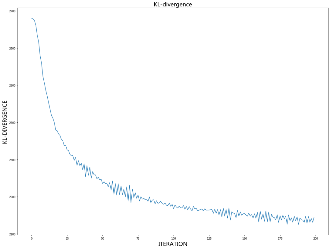
KL-散度看起来确实在优化过程逐渐减小，现在是时候显示低维嵌入的最终坐标 Y 了。

plt.figure(figsize=(16,12))
plt.scatter(y[:,0], y[:,1], c=y_train.astype(int), cmap = 'tab10', s = 20)
plt.title("tSNE on Cancer Associated Fibroblasts (CAFs): Programmed from Scratch", fontsize = 20)
plt.xlabel("tSNE1", fontsize = 20); 
plt.ylabel("tSNE2", fontsize = 20)
plt.show()

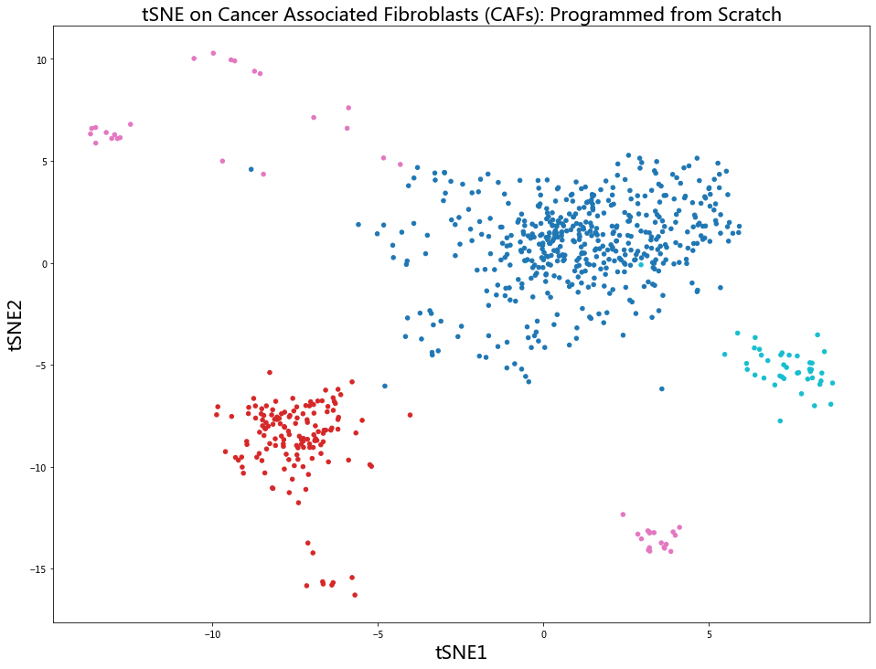
图中可见这些簇还是很明显的，但有些分散。

为了进行比较，我们还将运行 scikit-learn 中实现的 t-SNE 版本，以显示 t-SNE 用于数据 CAF 的典型效果。请注意，这是默认的 Barnes-Hut 实现，这意味着仅针对最近邻点计算高维概率，并且最近邻点的数量等于。另外，使用了参数 exaggeration = 12。所有这些小细节实际上在 t-SNE 的速度和可视化质量上都产生了很大的差异。

from sklearn.manifold import TSNE
model = TSNE(learning_rate = 100, n_components = 2, random_state = 123, perplexity = 30, verbose=2)
tsne = model.fit_transform(X_train)
plt.figure(figsize=(20, 15))
plt.scatter(tsne[:, 0], tsne[:, 1], c=y_train.astype(int), cmap = 'tab10', s = 50)
plt.title("tSNE on Cancer Associated Fibroblasts (CAFs): Burnes-Hut with Early Exaggeration", fontsize = 20)
plt.xlabel("tSNE1", fontsize = 20); plt.ylabel("tSNE2", fontsize = 20)
plt.show()

[t-SNE] Computing 91 nearest neighbors...
[t-SNE] Indexed 716 samples in 0.020s...
[t-SNE] Computed neighbors for 716 samples in 0.411s...
[t-SNE] Computed conditional probabilities for sample 716 / 716
[t-SNE] Mean sigma: 7.783218
[t-SNE] Computed conditional probabilities in 0.039s
[t-SNE] Iteration 50: error = 68.0411148, gradient norm = 0.4060098 (50 iterations in 0.072s)
[t-SNE] Iteration 100: error = 69.4176025, gradient norm = 0.3265068 (50 iterations in 0.069s)
[t-SNE] Iteration 150: error = 70.0493927, gradient norm = 0.3547082 (50 iterations in 0.116s)
[t-SNE] Iteration 200: error = 71.7179031, gradient norm = 0.3066460 (50 iterations in 0.068s)
[t-SNE] Iteration 250: error = 72.4487991, gradient norm = 0.3101583 (50 iterations in 0.067s)
[t-SNE] KL divergence after 250 iterations with early exaggeration: 72.448799
[t-SNE] Iteration 300: error = 1.4979095, gradient norm = 0.0030718 (50 iterations in 0.065s)
[t-SNE] Iteration 350: error = 1.3691742, gradient norm = 0.0008735 (50 iterations in 0.139s)
[t-SNE] Iteration 400: error = 1.3416479, gradient norm = 0.0003998 (50 iterations in 0.067s)
[t-SNE] Iteration 450: error = 1.3282142, gradient norm = 0.0003011 (50 iterations in 0.116s)
[t-SNE] Iteration 500: error = 1.3215110, gradient norm = 0.0001883 (50 iterations in 0.144s)
[t-SNE] Iteration 550: error = 1.3179287, gradient norm = 0.0001176 (50 iterations in 0.066s)
[t-SNE] Iteration 600: error = 1.3155496, gradient norm = 0.0001065 (50 iterations in 0.132s)
[t-SNE] Iteration 650: error = 1.3142179, gradient norm = 0.0000825 (50 iterations in 0.126s)
[t-SNE] Iteration 700: error = 1.3130822, gradient norm = 0.0000891 (50 iterations in 0.063s)
[t-SNE] Iteration 750: error = 1.3122742, gradient norm = 0.0000689 (50 iterations in 0.062s)
[t-SNE] Iteration 800: error = 1.3116283, gradient norm = 0.0000636 (50 iterations in 0.060s)
[t-SNE] Iteration 850: error = 1.3111641, gradient norm = 0.0000666 (50 iterations in 0.112s)
[t-SNE] Iteration 900: error = 1.3108296, gradient norm = 0.0000643 (50 iterations in 0.061s)
[t-SNE] Iteration 950: error = 1.3106019, gradient norm = 0.0000618 (50 iterations in 0.063s)
[t-SNE] Iteration 1000: error = 1.3102467, gradient norm = 0.0000535 (50 iterations in 0.061s)
[t-SNE] KL divergence after 1000 iterations: 1.310247

我们使用原始的 t-SNE 并设 early_exaggeration = 1。

from sklearn.manifold import TSNE
model = TSNE(learning_rate = 100, n_components = 2, 
             random_state = 123, perplexity = 30, early_exaggeration = 1, method = 'exact', verbose = 2)
tsne = model.fit_transform(X_train)
plt.figure(figsize=(20, 15))
plt.scatter(tsne[:, 0], tsne[:, 1], c=y_train.astype(int), cmap = 'tab10', s = 50)
plt.title("tSNE on Cancer Associated Fibroblasts (CAFs): Exact without Early Exaggeration", fontsize = 20)
plt.xlabel("tSNE1", fontsize = 20); plt.ylabel("tSNE2", fontsize = 20)
plt.show()

[t-SNE] Computing pairwise distances...
[t-SNE] Computed conditional probabilities for sample 716 / 716
[t-SNE] Mean sigma: 7.540113
[t-SNE] Iteration 50: error = 1.4848583, gradient norm = 0.0020657 (50 iterations in 0.713s)
[t-SNE] Iteration 100: error = 1.3750211, gradient norm = 0.0009555 (50 iterations in 0.718s)
[t-SNE] Iteration 150: error = 1.3380948, gradient norm = 0.0005748 (50 iterations in 0.693s)
[t-SNE] Iteration 200: error = 1.3188041, gradient norm = 0.0004392 (50 iterations in 0.713s)
[t-SNE] Iteration 250: error = 1.3050413, gradient norm = 0.0003492 (50 iterations in 0.692s)
[t-SNE] KL divergence after 250 iterations with early exaggeration: 1.305041
[t-SNE] Iteration 300: error = 1.2994059, gradient norm = 0.0002118 (50 iterations in 0.731s)
[t-SNE] Iteration 350: error = 1.2898256, gradient norm = 0.0001655 (50 iterations in 0.726s)
[t-SNE] Iteration 400: error = 1.2823523, gradient norm = 0.0001324 (50 iterations in 0.689s)
[t-SNE] Iteration 450: error = 1.2771731, gradient norm = 0.0001153 (50 iterations in 0.709s)
[t-SNE] Iteration 500: error = 1.2737796, gradient norm = 0.0000892 (50 iterations in 0.695s)
[t-SNE] Iteration 550: error = 1.2711932, gradient norm = 0.0000768 (50 iterations in 0.750s)
[t-SNE] Iteration 600: error = 1.2688715, gradient norm = 0.0000770 (50 iterations in 0.740s)
[t-SNE] Iteration 650: error = 1.2659149, gradient norm = 0.0000837 (50 iterations in 0.728s)
[t-SNE] Iteration 700: error = 1.2641687, gradient norm = 0.0000569 (50 iterations in 0.704s)
[t-SNE] Iteration 750: error = 1.2628826, gradient norm = 0.0000523 (50 iterations in 0.690s)
[t-SNE] Iteration 800: error = 1.2618663, gradient norm = 0.0000427 (50 iterations in 0.689s)
[t-SNE] Iteration 850: error = 1.2610543, gradient norm = 0.0000425 (50 iterations in 0.791s)
[t-SNE] Iteration 900: error = 1.2603252, gradient norm = 0.0000406 (50 iterations in 0.756s)
[t-SNE] Iteration 950: error = 1.2596114, gradient norm = 0.0000396 (50 iterations in 0.725s)
[t-SNE] Iteration 1000: error = 1.2588496, gradient norm = 0.0000419 (50 iterations in 0.717s)
[t-SNE] KL divergence after 1000 iterations: 1.258850

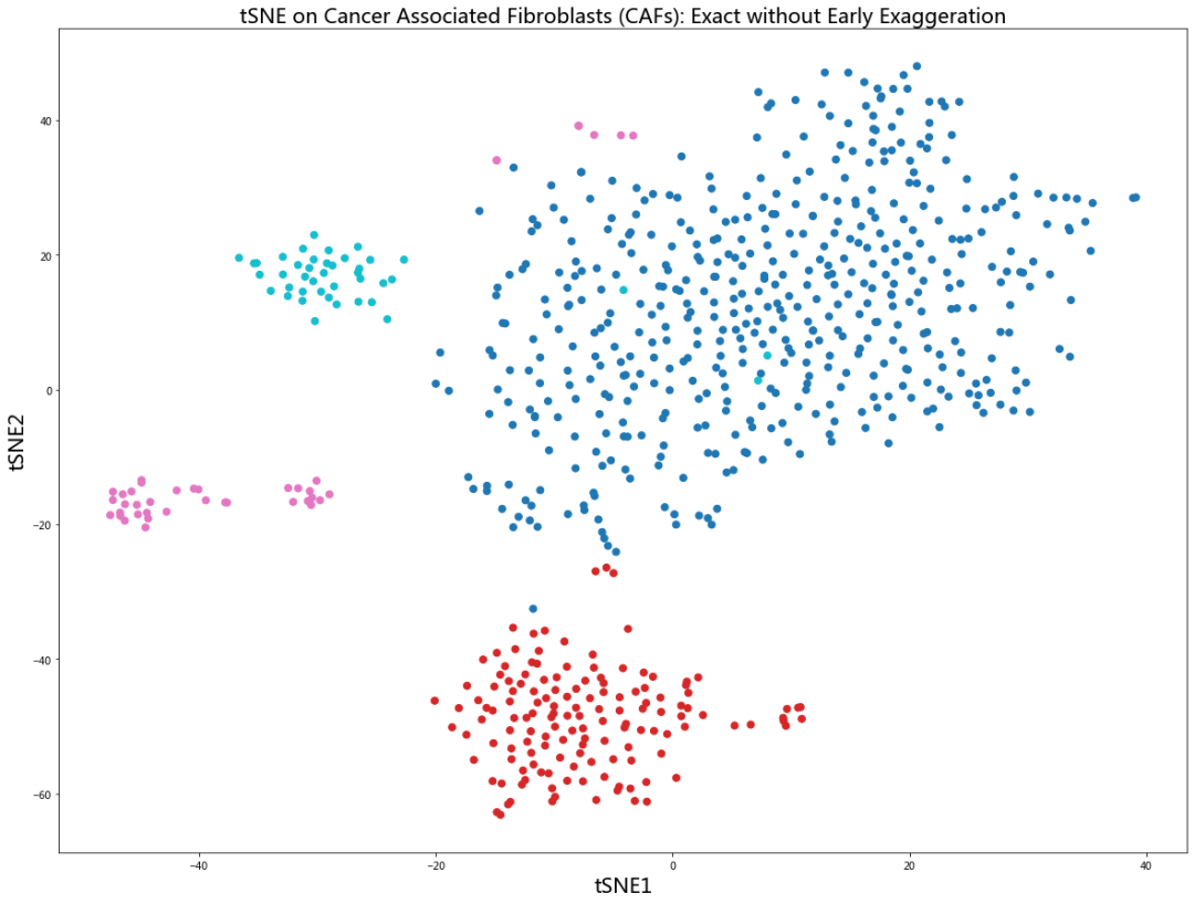
现在，各簇的分散变得更加明显，这类似于上面我们从头开始实现时的情况。请注意，平均 sigma 为 7.54，而在我们的实现中为 6.37。这是一个有趣的差异，将在后面消除。

.t-SNE 和 UMAP 的主要区别

UMAP 给我的第一印象是一种新的有趣的降维方法，与半靠数学理论半靠经验建立起来的算法 t-SNE 不同，UMAP 具有严格的数学理论背景。我的朋友告诉我原始 UMAP 论文^[4]太数学化了，看着论文的第 2 部分，我很高兴看到终于有严格而准确的数学理论应用到了数据科学中。阅读UMAP 文档^[5]并观看 Leland McInnes 在 SciPy 2018 上的演讲^[6]，我有点困惑并感觉到 UMAP 是另一种类似于 t-SNE 的技术，以致我难以理解 UMAP 与 t-SNE 到底有何不同。

从 UMAP 论文来看，即使 Lelan McInnes 试图在附录 C 中给出了总结，UMAP 和 t-SNE 之间的差异也不是很明显。我宁愿说，我确实看到了微小的差异，但尚不清楚为什么它们会有如此巨大的改进效果。在这里，我将首先总结我注意到的 UMAP 和 t-SNE 之间的差异，然后尝试解释这些差异为何如此重要，并弄清它们的影响有多大。

UMAP 在高维中使用指数概率，但不必像 t-SNE 那样使用欧几里德距离，而是使用任意距离度量。此外，概率并未归一化处理，

p_{i|j} = \displaystyle \large{e}^{\small - \displaystyle \frac{d(x_i, x_j) - \rho_i}{\sigma_i}}

这里是一个非常重要的参数，代表每个数据点到其最近邻近点的距离。这提供了流形的局部连接。换句话说，这为每个数据点施加了一个局部可自我调整的指数核，因此每个数据点上的距离度量可以不同。

UMAP 没有对高维或低维概率应用归一化，这与 t-SNE 有很大不同，这点貌似有些奇怪。但是，仅从高维或低维概率的函数形式可以看出，它们已经针对区间 [0,1] 进行了缩放，因此跳过归一化可能很好。然而，事实证明等式中缺乏归一化，公式 (1) 中的分母，大大减少了高维图的计算时间。
UMAP 使用最近相邻点的数量而不是困惑度。虽然 t-SNE 将困惑度定义为，，但 UMAP 定义了不需要函数的最近相邻点的数量 k，即，

k = {2}^{\small \displaystyle \sum_i p_{ij}}

UMAP 对的对称化略有不同。对称是必要的，因为在 UMAP 将具有局部变化的度量的点粘合在一起之后，可能会发生两个节点 A 和 B 之间的图的权重为的情况。

p_{ij} = p_{i|j} + p_{j|i} - p_{i|j}p_{j|i}

UMAP 使用函数族来表示低维度上的距离概率，不是学生 t-分布，但是也非常相似，请再次注意没有使用规一化，

q_{ij} = \left ( 1 + a(y_i - y_j) ^{2b} \right ) ^ {-1},

其中，和为默认的 UMAP 超参数。实际上，UMAP 从非线性最小二乘拟合中找到和，

\left ( 1 + a(y_i - y_j) ^{2b} \right ) ^ {-1} \approx \begin{cases} 1 & \text{if } y_i - y_j\le \rm{min\_dist}\\ e^{\displaystyle -(y_i - y_j) - \rm{min\_dist}} & \text{if } y_i - y_j >\rm{min\_dist} \end{cases} \hspace{2em} (5)

为了更好地理解曲线族的性质，让我们来画一些看:

plt.figure(figsize=(20, 15))
y = np.linspace(0, 10, 1000)

my_prob = lambda y, a, b: np.power(1 + ay(2b), -1)
plt.plot(y, my_prob(y, a = 1, b = 1))
plt.plot(y, my_prob(y, a = 1.93, b = 0.79))
plt.plot(y, my_prob(y, a = 1.93, b = 5))

plt.gca().legend(('a = 1, b = 1', 'a = 1.93, b = 0.79', 'a = 1.93, b = 5'), fontsize = 20)
plt.title("Low-Dimensional Probability of Pairwise Euclidean Distances", fontsize = 20)
plt.xlabel("Y", fontsize = 20); plt.ylabel("Q(Y)", fontsize = 20)
plt.show()

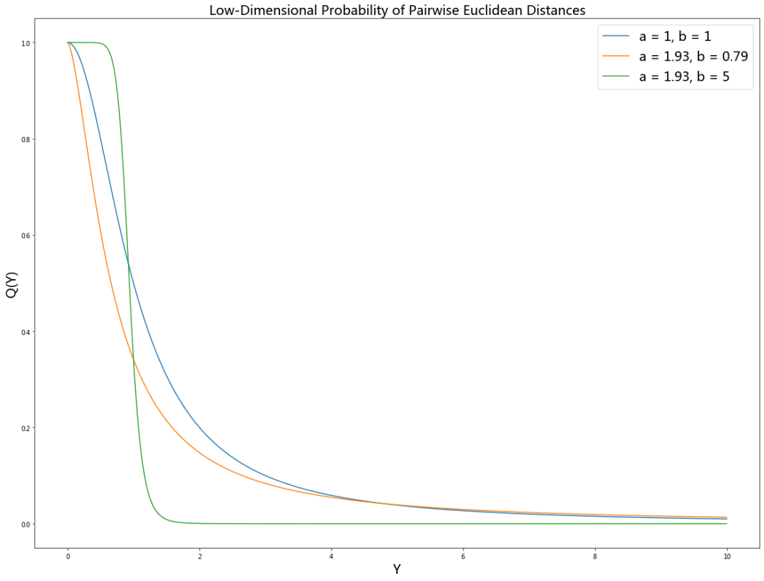
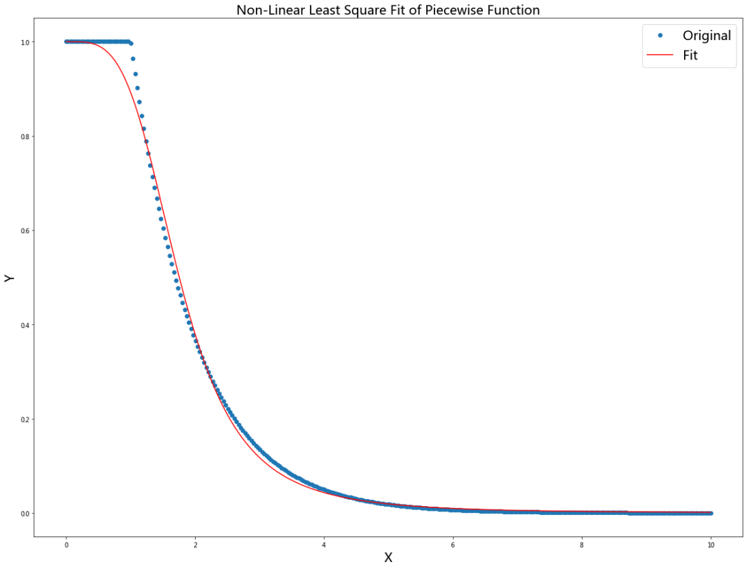
我们可以看到曲线族对参数非常敏感，在较大时，曲线在较小时形成平稳状态。这意味着在 UMAP 超参数 min_dist 下，所有数据点均紧紧相关连接的。由于函数的行为几乎类似于 Heaviside step 函数^[7]，因此这意味着 UMAP 为低维空间中彼此靠近的所有点分配几乎相同的低维坐标。min_dist 正是导致通常在 UMAP 降维图中经常观察到的超紧密堆积簇的原因。

为了证明公式 (5) 的拟合度到底如何，让我们绘制一个简单的分段函数（图中平坦区域由 min_dist 参数定义），并通过 python 库 scipy 中的 optimize.curve_fit 函数对其用函数族进行拟合。拟合的结果是，我们为函数获得了优化的参数 a 和 b。

from scipy import optimize
import matplotlib.pyplot as plt
import numpy as np

MIN_DIST = 1

x = np.linspace(0, 10, 300)

def f(x, min_dist):
    y = []
    for i in range(len(x)):
        if(x[i] <= min_dist):
            y.append(1)
        else:
            y.append(np.exp(- x[i] + min_dist))
    return y

dist_low_dim = lambda x, a, b: 1 / (1 + ax(2b))
    
p , _ = optimize.curve_fit(dist_low_dim, x, f(x, MIN_DIST))
print(p)

plt.figure(figsize=(20,15))
plt.plot(x, f(x, MIN_DIST), "o")
plt.plot(x, dist_low_dim(x, p[0], p[1]), c = "red")
plt.title("Non-Linear Least Square Fit of Piecewise Function", fontsize = 20)
plt.gca().legend(('Original', 'Fit'), fontsize = 20)
plt.xlabel("X", fontsize = 20)
plt.ylabel("Y", fontsize = 20)
plt.show()

[0.12015106 1.88131742]

UMAP 使用二元交叉熵（CE） 作为代价函数，而不是像 t-SNE 那样使用 KL-散度。

\text{CE} (X, Y) = \sum_i \sum_j \left[ p_{ij}(X) \log \left(\frac {p_{ij}(X)} {q_{ij}(Y)}\right) + \left(1- p_{ij}(X)\right) \log \left(\frac {1 - p_{ij}(X)} {1 - q_{ij}(Y)}\right) \right]

在下一节中，我们将显示 CE 代价函数中的附加（第二）项使得 UMAP 能够捕获全局结构，而 t-SNE 只能将局部结构保留为中等的困惑度值。有趣的是，为什么 UMAP 使用二元交叉熵，通常将其用于区分两类物体（例如猫与狗）的分类问题。在这里，是对任何数值进行分类，而且它不是二分类问题。

为了使用梯度下降法，我们需要快速计算交叉熵的梯度。忽略仅包含的常数项，我们可以重写交叉熵并求导，

\text{CE}(X, d_{ij}) = \sum_j \left[ -P(X)\log Q(d_{ij}) + \left(1-P(X)\right)\log\left(1 - Q(d_{ij})\right)\right], \hspace{0.85em}\text{其中}\; d_{ij} = y_i - y_j

Q(d_{ij}) = \frac{1}{1 + a d_{ij}^{2b}}; \hspace{0.5em} 1 - Q(d_{ij}) = \frac{a d_{ij}^{2b}}{1 + a d_{ij}^{2b}}; \hspace{0.5em} \frac{\delta Q}{\delta d_{ij}} = -\frac{2ab d_{ij}^{2b-1}}{\left(1 + a d_{ij}^{2b}\right)^2}

\begin{array}{lll} \dfrac{\delta \text{CE}}{\delta y_i} &= \sum_j \left[ -\dfrac{P(X)}{Q(d_{ij})}\dfrac{\delta Q}{\delta d_{ij}} + \dfrac{1 - P(X)}{1 - Q(d_{ij})}\dfrac{\delta Q}{\delta d_{ij}} \right] \\[0.8em]&= \sum_j \left[ \left(-P(X)\left(1 + a d_{ij}^{2b}\right) + \dfrac{(1-P(X))\left(1 + a d_{ij}^{2b}\right)}{\left(a d_{ij}^{2b}\right)} \right)\dfrac{\delta Q}{\delta d_{ij}} \right] \end{array}

\dfrac{\delta \text{CE}}{\delta y_i} = \sum_j \left[ \dfrac{2abd_{ij}^{2(b-1)}P(X)}{1 + a d_{ij}^{2b}} - \dfrac{2b(1-P(X))}{d_{ij}^2(1 + a d_{ij}^{2b})} \right]\left(y_i - y_j\right) \hspace{2em} (6)

与 t-SNE 使用的随机正态初始化相比，UMAP 使用图 Laplacian 初始化低维坐标。但是，这应该对最终的低维表示形式影响较小，至少对于 t-SNE 来说是这样的^[8]。但是，这将使 UMAP 在每次运行之间的更改减少，因为它不再是随机初始化了。Linderman and Steinerberger 的假设^[9]启发了通过图拉普拉斯算子进行初始化的选择，他们建议在最小化 KL-散度时，初始化作一定夸大等同于构造图 Laplacian。

图拉普拉斯算子、谱聚类、拉普拉斯算子特征图、扩散图、谱嵌入等实际上都是指将矩阵分解和邻接图方法相结合以解决降维问题的有趣方法。在这种方法中，我们从构造一个图（或 knn-graph）开始，并通过构造拉普拉斯矩阵，即用矩阵代数（邻接矩阵和度矩阵）对其进行公式化，最后将拉普拉斯矩阵分解，即解决特征值分解问题。

L = D^{1/2}\left(D - A\right)D^{1/2}

我们可以使用 Python 库 scikit-learn（该库的快速入门请看本号此篇）中的 SpectralEmbedding 函数来初始化低维坐标。

from sklearn.manifold import SpectralEmbedding

model = SpectralEmbedding(n_components = 2, n_neighbors = 50)
se = model.fit_transform(np.log(X_train + 1))

plt.figure(figsize=(20,15))
plt.scatter(se[:, 0], se[:, 1], c = y_train.astype(int), cmap = 'tab10', s = 50)
plt.title('Laplacian Eigenmap', fontsize = 20)
plt.xlabel("LAP1", fontsize = 20)
plt.ylabel("LAP2", fontsize = 20)
plt.show()

.为什么 t-SNE 仅保留局部结构？

现在让我们简短地讨论一下为什么有人说 t-SNE 只保留数据的局部结构。可以从不同的角度理解 t-SNE 的局部性。首先，我们在式 (1) 中有参数，它设置我们的数据点在如何相互局部感知对方。由于成对的欧几里得距离的概率呈指数下降，因此在较小的地方，它对于远点（大）基本上为零，而对于邻近点（小）则迅速增长。相反，当大的地方，远近点的概率差距变得没那么剧烈了，当趋于无穷大时，即，对任何点对之间的所有距离，概率都等于 1，相当于点变得等距。

plt.figure(figsize=(20, 15))
x = np.linspace(0, 10, 1000)
sigma_list = [0.1, 1, 5, 10]

for sigma in sigma_list:
    my_prob = lambda x: np.exp(-x2 / (2*sigma2))
    plt.plot(x, my_prob(x))
plt.gca().legend(('$\sigma$ = 0.1','$\sigma$ = 1', '$\sigma$ = 5', '$\sigma$ = 10'), fontsize = 20)
plt.title("High-Dimensional Probability of Pairwise Euclidean Distances", fontsize = 20)
plt.xlabel("X", fontsize = 20); plt.ylabel("P(X)", fontsize = 20)
plt.show()

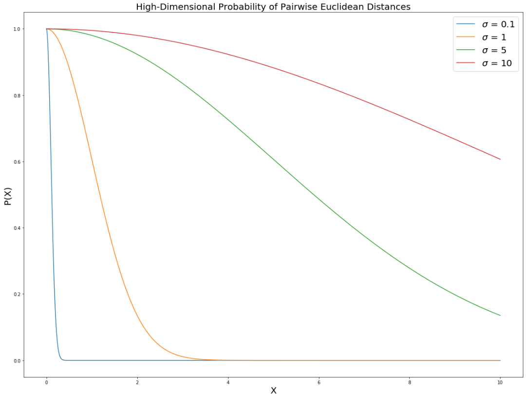
有趣的是，如果我们将高维空间中成对的欧几里得距离的概率在处泰勒展开，我们将得到二阶逼近的幂定律：

P(X) \approx \displaystyle e^{\displaystyle -\frac{X^2}{2\sigma^2}}

P(X) \underset{\displaystyle\sigma\rightarrow \infty}{\longrightarrow} 1 - \frac{X^2}{2\sigma^2} + \frac{X^4}{8\sigma^4} - \dots \hspace{2em} (7)

关于成对点的欧几里得距离的幂定律类似于多维尺度（MDS）算法^[10]的代价函数，已知该函数通过尝试保持对点之间的距离来保持全局结构，即无论它们相距远还是近。可以用以下方式解释这一点：对于大，t-SNE 确实也兼顾了点之间的远程交互作用，因此说 t-SNE 仅可以处理局部距离并不完全正确。但是，我们通常使用较小的困惑度，就像 Laurens van der Maaten 建议的困惑度在 5 到 50 之间^[11]，尽管也许局部和全局之间本可以很好地采取折衷办法，即根据平方根法则 ^[12] 来近似选择困惑度，其中 N 是样本大小。

另一方面，在高维概率的行为中导致极端的局部性，类似于狄拉克函数。

P(X) \underset{\displaystyle\sigma\rightarrow 0}{\longrightarrow} \delta_{\sigma}(X) \hspace{2em} (8)

解释 t-SNE 的局部性的另一种方法是考虑 KL-散度函数。让我们尝试绘制它，假设 X 是高维空间中点之间的距离，而 Y 是低维距离：

P(X) \approx e^{\displaystyle - X^2} \hspace{2em} Q(Y) \approx \frac{1}{1+Y^2}

从公式 (4) KL-散度的定义知：

\text{KL}(X,Y) = P(X)\log\left(\frac{P(X)}{Q(Y)}\right) = P(X)\log P(X) - P(X)\log Q(Y) \hspace{2em} (9)

等式 (9) 中的第一项，不管大的 X 还是小的 X，它都接近于零。对于小 X 而言，它接近于零，是因为指数变得接近于 1，而。对于大的 X，该项仍为零，因为变为零的速度比到达来得更快。因此，为了直观地理解 KL-散度，仅考虑第二项就足够了：

\text{KL}(X,Y) \approx - P(X)\log Q(Y) = e^{\displaystyle - X^2} \log \left(1 + Y^2\right)

这是一个看起来很奇怪的函数，让我们绘制：

import numpy as np
import matplotlib.pyplot as plt
from matplotlib import cm
from mpl_toolkits.mplot3d import Axes3D
from matplotlib.ticker import LinearLocator, FormatStrFormatter

fig = plt.figure(figsize=(20, 15))
ax = fig.gca(projection = '3d')
# Set rotation angle to 30 degrees
ax.view_init(azim=30)

X = np.arange(0, 3, 0.1)
Y = np.arange(0, 3, 0.1)
X, Y = np.meshgrid(X, Y)
Z = np.exp(-X2)*np.log(1 + Y2)

# Plot the surface.
surf = ax.plot_surface(X, Y, Z, cmap=cm.coolwarm,linewidth=0, antialiased=False)
ax.set_xlabel('X', fontsize = 20)
ax.set_ylabel('Y', fontsize = 20)
ax.set_zlabel('KL (X, Y)', fontsize = 20)
ax.set_zlim(0, 2.2)
ax.zaxis.set_major_locator(LinearLocator(10))
ax.zaxis.set_major_formatter(FormatStrFormatter('%.02f'))

# Add a color bar which maps values to colors.
fig.colorbar(surf, shrink=0.5, aspect=5)
plt.show()

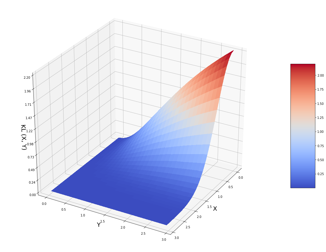
该函数具有非常不对称的形状。如果高维中的点之间的距离 X 小，则指数前置因子为 1，对数项的行为与相同，这意味着，如果低维 Y 的距离较大，则将存在一个高惩罚，因此 t-SNE 尝试在小 X 处减小 Y，以减小惩罚。但是，对于高维空间的长距离 X，Y 基本上可以取从 0 到的任何值，因为指数项变为 0 并且总是胜过对数项。因此，可能会发生在高维度上相距较远的点最终在低维度上彼此接近的情况。换句话说，t-SNE 不保证在高维上相距较远的点在低维上也保持相距较远。但是，它确实保证了在高维度上彼此靠近的点在低维度上仍将彼此靠近。因此它仅保留局部数据结构，前提是不使用 。

.为什么 UMAP 可以保全局结构

与 t-SNE 相比，UMAP 使用交叉熵（CE）作为代价函数，而不是 KL-散度为，

\text{CE}(X,Y) = P(X)\log\left(\frac{P(X)}{Q(Y)}\right) + \left(1-P(X)\right)\log\left(\frac{1-P(X)}{1-Q(Y)}\right)

\text{CE}(X, Y) = e^{\displaystyle - X^2} \log \left[e^{\displaystyle - X^2}\left(1 + Y^2\right)\right] + \left(1 - e^{\displaystyle - X^2}\right) \log \left[\frac{\left(1-e^{\displaystyle - X^2}\right)\left(1 + Y^2\right)}{Y^2}\right]\\[1.8em] \approx e^{\displaystyle - X^2} \log \left(1 + Y^2\right) + \left(1-e^{\displaystyle - X^2}\right) \log \left(\frac{1 + Y^2}{Y^2}\right)

这导致在局部-全局结构保存平衡的性能上的巨大变化。在 X 的较小值处，我们获得与 t-SNE 相同的约束，因为第二项由于前置因子以及对数函数比多项式函数更慢趋于 0 的事实而几乎可以忽略：

X\rightarrow 0: \text{CE}(X, Y) \approx \log \left(1 + Y^2\right)

因此，为了使惩罚最小化，必须让 Y 也变得小，即。这与 t-SNE 的行为完全一样。

但是，在 X 值很大的时候（即），第一项几乎可以忽略了，而第二项的前置因子变为 1，于是得到：

X\rightarrow \infty: \text{CE}(X, Y) \approx \log \left(\frac{1 + Y^2}{Y^2}\right)

在这里，如果 Y 小，由于括号里分母变得很大，代价函数值变得较高，因此鼓励 Y 值较大，以使得括号中分数接近 1，那么代价函数值讲接近于 0。此时，在处得到了。因此，从高维空间移动到低维空间时，全局距离（大的）得以保留，这正是我们想要的。

为了说明这一点，让我们把 UMAP 的 CE 代价函数绘制出来看看：

?import numpy as np
import matplotlib.pyplot as plt
from matplotlib import cm
from mpl_toolkits.mplot3d import Axes3D
from matplotlib.ticker import LinearLocator, FormatStrFormatter

fig = plt.figure(figsize=(20, 15))
ax = fig.gca(projection = '3d') 
# Set rotation angle to 30 degrees
ax.view_init(azim=30)

X = np.arange(0, 3, 0.001)
Y = np.arange(0, 3, 0.001)
X, Y = np.meshgrid(X, Y)
Z = np.exp(-X2)np.log(1 + Y2) + (1 - np.exp(-X2))np.log((1 + Y2) / (Y**2+0.01))

# Plot the surface.
surf = ax.plot_surface(X, Y, Z, cmap=cm.coolwarm,linewidth=0, antialiased=False)
ax.set_xlabel('X', fontsize = 20)
ax.set_ylabel('Y', fontsize = 20)
ax.set_zlabel('CE (X, Y)', fontsize = 20)
ax.set_zlim(0, 4.3)
ax.zaxis.set_major_locator(LinearLocator(10))
ax.zaxis.set_major_formatter(FormatStrFormatter('%.02f'))

# Add a color bar which maps values to colors.
fig.colorbar(surf, shrink=0.5, aspect=5)
plt.show()

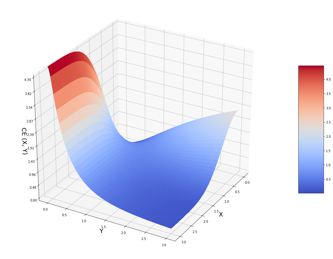
在这里，我们看到该图的右侧部分看上去与上面的 KL-散度表现非常相似。意味着在 X 较小的地方，我们仍然希望将 Y 减小以减少惩罚。但是，在 X 大的地方，Y 的距离也确实想变大，因为如果变小，则的代价将很大。请记住，以前，对于曲面，在大 X 处 Y 值的大小对惩罚来说没有任何区别。这就是为什么代价函数能够保留全局距离和局部距离的原因。

.从头开始编写 UMAP

我们前面已经从头实现过 t-SNE，现在也了解 t-SNE 和 UMAP 之间的关键区别。下面我们尝试通过修改 t-SNE 代码来从头实现 UMAP 算法。

import numpy as np
import pandas as pd
from scipy import optimize
import matplotlib.pyplot as plt
from sklearn.manifold import SpectralEmbedding
from sklearn.metrics.pairwise import euclidean_distances

path = './'
expr = pd.read_csv(path + 'CAFs.txt', sep='\t')
print(expr.iloc[0:4,0:4])
X_train = expr.values[:,0:(expr.shape[1]-1)]
X_train = np.log(X_train + 1)
n = X_train.shape[0]
print("\nThis data set contains " + str(n) + " samples")
y_train = expr.values[:,expr.shape[1]-1]
print("\nDimensions of the  data set: ")
print(X_train.shape, y_train.shape)

                1110020A21Rik  1110046J04Rik  1190002F15Rik  1500015A07Rik
SS2_15_0048_A3            0.0            0.0            0.0            0.0
SS2_15_0048_A6            0.0            0.0            0.0            0.0
SS2_15_0048_A5            0.0            0.0            0.0            0.0
SS2_15_0048_A4            0.0            0.0            0.0            0.0

This data set contains 716 samples

Dimensions of the  data set: 
(716, 557) (716,)

dist = np.square(euclidean_distances(X_train, X_train))
rho = [sorted(dist[i])[1] for i in range(dist.shape[0])]
print(dist[0:4, 0:4])
print('\n')
print(rho[0:4])

[[  0. 144. 206. 146.]
 [144.   0. 216. 180.]
 [206. 216.   0. 164.]
 [146. 180. 164.   0.]]


[63.0, 41.999996, 96.00001, 16.0]

def prob_high_dim(sigma, dist_row):
    """
    For each row of Euclidean distance matrix (dist_row) compute
    probability in high dimensions (1D array)
    """
    d = dist[dist_row] - rho[dist_row]
    d[d < 0] = 0
    return np.exp(- d / sigma)

def k(prob):
    """
    Compute n_neighbor = k (scalar) for each 1D array of high-dimensional probability
    """
    return np.power(2, np.sum(prob))

def sigma_binary_search(k_of_sigma, fixed_k):
    """
    Solve equation k_of_sigma(sigma) = fixed_k 
    with respect to sigma by the binary search algorithm
    """
    sigma_lower_limit = 0
    sigma_upper_limit = 1000
    for i in range(20):
        approx_sigma = (sigma_lower_limit + sigma_upper_limit) / 2
        if k_of_sigma(approx_sigma) < fixed_k:
            sigma_lower_limit = approx_sigma
        else:
            sigma_upper_limit = approx_sigma
        if np.abs(fixed_k - k_of_sigma(approx_sigma)) <= 1e-5:
            break
    return approx_sigma

N_NEIGHBOR = 15
prob = np.zeros((n,n))
sigma_array = []
for dist_row in range(n):
    func = lambda sigma: k(prob_high_dim(sigma, dist_row))
    binary_search_result = sigma_binary_search(func, N_NEIGHBOR)
    prob[dist_row] = prob_high_dim(binary_search_result, dist_row)
    sigma_array.append(binary_search_result)
    if (dist_row + 1) % 100 == 0:
        print("Sigma binary search finished {0} of {1} cells".format(dist_row + 1, n))
print("\nMean sigma = " + str(np.mean(sigma_array)))

Sigma binary search finished 100 of 2500 cells
Sigma binary search finished 200 of 2500 cells
Sigma binary search finished 300 of 2500 cells
Sigma binary search finished 400 of 2500 cells
Sigma binary search finished 500 of 2500 cells
Sigma binary search finished 600 of 2500 cells
Sigma binary search finished 700 of 2500 cells
Sigma binary search finished 800 of 2500 cells
Sigma binary search finished 900 of 2500 cells
Sigma binary search finished 1000 of 2500 cells
Sigma binary search finished 1100 of 2500 cells
Sigma binary search finished 1200 of 2500 cells
Sigma binary search finished 1300 of 2500 cells
Sigma binary search finished 1400 of 2500 cells
Sigma binary search finished 1500 of 2500 cells
Sigma binary search finished 1600 of 2500 cells
Sigma binary search finished 1700 of 2500 cells
Sigma binary search finished 1800 of 2500 cells
Sigma binary search finished 1900 of 2500 cells
Sigma binary search finished 2000 of 2500 cells
Sigma binary search finished 2100 of 2500 cells
Sigma binary search finished 2200 of 2500 cells
Sigma binary search finished 2300 of 2500 cells
Sigma binary search finished 2400 of 2500 cells
Sigma binary search finished 2500 of 2500 cells

Mean sigma = 5.911624145507813

#P = prob + np.transpose(prob) - np.multiply(prob, np.transpose(prob))
P = (prob + np.transpose(prob)) / 2

MIN_DIST = 0.25

x = np.linspace(0, 3, 300)

def f(x, min_dist):
    y = []
    for i in range(len(x)):
        if(x[i] <= min_dist):
            y.append(1)
        else:
            y.append(np.exp(- x[i] + min_dist))
    return y

dist_low_dim = lambda x, a, b: 1 / (1 + ax(2b))

p , _ = optimize.curve_fit(dist_low_dim, x, f(x, MIN_DIST))

a = p[0]
b = p[1] 
print("Hyperparameters a = " + str(a) + " and b = " + str(b))

Hyperparameters a = 1.121436342369708 and b = 1.057499876613678

a = 1
b = 1

def prob_low_dim(Y):
    """
    Compute matrix of probabilities q_ij in low-dimensional space
    """
    inv_distances = np.power(1 + a  np.square(euclidean_distances(Y, Y))*b, -1)
    return inv_distances
def CE(P, Y):
    """
    Compute Cross-Entropy (CE) from matrix of high-dimensional probabilities 
    and coordinates of low-dimensional embeddings
    """
    Q = prob_low_dim(Y)
    return - P  np.log(Q + 0.01) - (1 - P)  np.log(1 - Q + 0.01)

def CE_gradient(P, Y):
    """
    Compute the gradient of Cross-Entropy (CE)
    """
    y_diff = np.expand_dims(Y, 1) - np.expand_dims(Y, 0)
    inv_dist = np.power(1 + a  np.square(euclidean_distances(Y, Y))*b, -1)
    Q = np.dot(1 - P, np.power(0.001 + np.square(euclidean_distances(Y, Y)), -1))
    np.fill_diagonal(Q, 0)
    Q = Q / np.sum(Q, axis = 1, keepdims = True)
    fact = np.expand_dims(a  P  (1e-8 + np.square(euclidean_distances(Y, Y)))**(b-1) - Q, 2)
    return 2  b  np.sum(fact  y_diff  np.expand_dims(inv_dist, 2), axis = 1)

N_LOW_DIMS = 2
LEARNING_RATE = 1
MAX_ITER = 200

np.random.seed(12345)
model = SpectralEmbedding(n_components = N_LOW_DIMS, n_neighbors = 20)
y = model.fit_transform(np.log(X_train + 1))
#y = np.random.normal(loc = 0, scale = 1, size = (n, N_LOW_DIMS))

CE_array = []
print("Running Gradient Descent: \n")
for i in range(MAX_ITER):
    y = y - LEARNING_RATE * CE_gradient(P, y)
    
    plt.figure(figsize=(20,15))
    plt.scatter(y[:,0], y[:,1], c = y_train.astype(int), cmap = 'tab10', s = 50)
    plt.title("UMAP on Cancer Associated Fibroblasts (CAFs): Programmed from Scratch", fontsize = 20)
    plt.xlabel("UMAP1", fontsize = 20); plt.ylabel("UMAP2", fontsize = 20)
    plt.savefig('./UMAP_Plots/UMAP_iter_' + str(i) + '.png')
    plt.close()
    
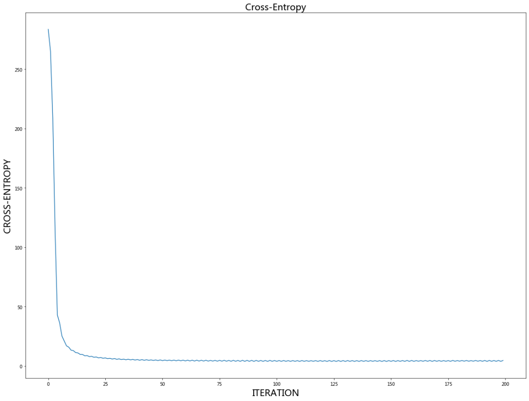
    CE_current = np.sum(CE(P, y)) / 1e+5
    CE_array.append(CE_current)
    if i % 10 == 0:
        print("Cross-Entropy = " + str(CE_current) + " after " + str(i) + " iterations")

Running Gradient Descent: 

Cross-Entropy = 283.5777742781302 after 0 iterations
Cross-Entropy = 13.268591570309042 after 10 iterations
Cross-Entropy = 7.259540019861242 after 20 iterations
Cross-Entropy = 5.585781444474118 after 30 iterations
Cross-Entropy = 4.790947502899679 after 40 iterations
Cross-Entropy = 4.461962382188084 after 50 iterations
Cross-Entropy = 4.230262677049629 after 60 iterations
Cross-Entropy = 4.07024828797863 after 70 iterations
Cross-Entropy = 3.919821089922779 after 80 iterations
Cross-Entropy = 3.8173389159808866 after 90 iterations
Cross-Entropy = 3.8685463789976953 after 100 iterations
Cross-Entropy = 3.7978578320444876 after 110 iterations
Cross-Entropy = 3.855574433730828 after 120 iterations
Cross-Entropy = 3.766086348188088 after 130 iterations
Cross-Entropy = 3.8250638958646865 after 140 iterations
Cross-Entropy = 3.847715728119791 after 150 iterations
Cross-Entropy = 3.843081982582799 after 160 iterations
Cross-Entropy = 3.8990071294477766 after 170 iterations
Cross-Entropy = 3.993608725933739 after 180 iterations
Cross-Entropy = 3.9034721312778835 after 190 iterations

plt.figure(figsize=(20,15))
plt.plot(CE_array)
plt.title("Cross-Entropy", fontsize = 20)
plt.xlabel("ITERATION", fontsize = 20); plt.ylabel("CROSS-ENTROPY", fontsize = 20)
plt.show()

plt.figure(figsize=(20,15))
plt.scatter(y[:,0], y[:,1], c = y_train.astype(int), cmap = 'tab10', s = 50)
plt.title("UMAP on Cancer Associated Fibroblasts (CAFs): Programmed from Scratch", fontsize = 20)
plt.xlabel("UMAP1", fontsize = 20); plt.ylabel("UMAP2", fontsize = 20)
plt.show()

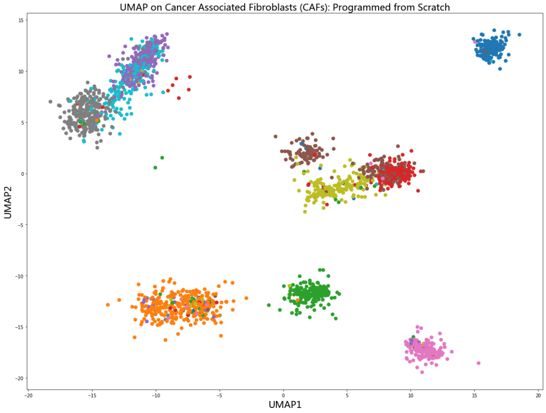
如图所示，在 UMAP 绘制图中往往可以看到各自紧紧簇拥的不同簇。而且，这些数据簇现在可以使用任意的聚类算法（基于图或基于密度）来作聚类处理，即使是 K-均值（k-mean）或高斯混合模型（GMM）在如此清晰的降维图上也能很好地完成任务。

为了检验我们实现的效果，让我们使用 UMAP 作者 Leland McInnes 实现的 Python 版本^[13]和相同的超参数与我们从头实现的版本进行比较：

from umap import UMAP
plt.figure(figsize=(20,15))
model = UMAP(n_neighbors = 15, min_dist = 0.25, n_components = 2, verbose = True)
umap = model.fit_transform(X_train)
plt.scatter(umap[:, 0], umap[:, 1], c = y_train.astype(int), cmap = 'tab10', s = 50)
plt.title('UMAP', fontsize = 20)
plt.xlabel("UMAP1", fontsize = 20)
plt.ylabel("UMAP2", fontsize = 20)
plt.show()

UMAP(a=None, angular_rp_forest=False, b=None,
     force_approximation_algorithm=False, init='spectral', learning_rate=1.0,
     local_connectivity=1.0, low_memory=False, metric='euclidean',
     metric_kwds=None, min_dist=0.25, n_components=2, n_epochs=None,
     n_neighbors=15, negative_sample_rate=5, output_metric='euclidean',
     output_metric_kwds=None, random_state=None, repulsion_strength=1.0,
     set_op_mix_ratio=1.0, spread=1.0, target_metric='categorical',
     target_metric_kwds=None, target_n_neighbors=-1, target_weight=0.5,
     transform_queue_size=4.0, transform_seed=42, unique=False, verbose=True)
Construct fuzzy simplicial set
Tue Jun 16 10:30:29 2020 Finding Nearest Neighbors
Tue Jun 16 10:30:30 2020 Finished Nearest Neighbor Search
Tue Jun 16 10:30:32 2020 Construct embedding
	completed  0  /  500 epochs
	completed  50  /  500 epochs
	completed  100  /  500 epochs
	completed  150  /  500 epochs
	completed  200  /  500 epochs
	completed  250  /  500 epochs
	completed  300  /  500 epochs
	completed  350  /  500 epochs
	completed  400  /  500 epochs
	completed  450  /  500 epochs
Tue Jun 16 10:30:34 2020 Finished embedding

我们得出的结论是，作者 Leland McInnes 实现的 UMAP 版本与我们从头实现的版本效果上非常相似。从某种意义上说，我们降维结果中的簇看起来更加紧致。通过设置 a = 1 和 b = 1（如学生 t-分布）和使用 t-SNE 对称化，而不是 UMAP 算法中使用 Hadamard 乘积的对称化，效果上可以略微比原始 UMAP 版本好一点。

我的预测是 UMAP 仅仅是开始，将来会有更多更好的降维技术，因为调整低/高维分布、进行更好的归一化、更好的代价函数、利用吸引力/排斥力解决 N 体问题等等技术手段，或许可以获得更好的低维表示。我希望在单细胞研究领域能够大量使用此类技术，因为即使通过少量修改，我也可以改善 UMAP 的低维表示。

.UMAP 为何比 t-SNE 快呢？

我们知道在涉及大量样本，嵌入维度的数量大于 2 和 3，原始数据中存在大量外围维度时，UMAP 比 t-SNE 运行得更快。

让我们尝试从数学原理和算法实现中了解为什么 UMAP 相对于 t-SNE 具有优越性。t- SNE 和 UMAP 基本上都包含两个步骤。

构建高维图，并使用二分搜索和固定最近邻点的数量来确定指数概率中的带宽。
通过梯度下降法优化低维嵌入。第二步是算法的瓶颈，因为前后步骤之间是连贯的，并且不能通过多线程优化^[14]。

但是，我注意到 UMAP 的第一步比 t-SNE 快得多。这里有两个原因，

首先，我们在定义最近邻居数的定义中删除了求对数部分，即不像 t-SNE 那样计算熵的完整公式：

k = 2^{\small \displaystyle \sum_i p_{ij}}

由于算法上的对数函数是通过泰勒级数展开来计算的，但是实际上将对数放在线性项的前面并不会增加多少值。因为对数函数比线性函数要慢得多，因此完全略过此步骤是很好的选择。

再者，是我们省略了像 t-SNE 那样在式 (1) 中对高维概率的归一化。这个具有争议性的骚操作实际上对性能产生了极大影响。这是因为求和或积分是一个计算开销很大的步骤。想一想贝叶斯法则中的分母归一化及其计算难度。通常，使用马尔可夫链蒙特卡罗方法（Markov Chain Monte Carlo，简称 MCMC）来近似计算该积分。虽然在 t-SNE 中的求和部分更易于分析计算，但毕竟涉及指数函数，仍然是消耗计算的步骤，因此跳过此步骤可以显著加快 UMAP 的第一阶段。

另外，UMAP 实际上也提高了第二步的速度。这方面的改进主要有这几个原因:

跟 t-SNE 或 FIt-SNE 不同的是，UMAP 使用了随机梯度下降（SGD）来代替常规的梯度下降（GD）。这极大地提高了速度，因为对于 SGD，你可以从随机样本子集计算梯度，而不是像常规 GD 一样需要一次性使用所有样本。除了提高速度外，这还减少了内存消耗，因为不必为内存中的所有样本保留梯度，而仅保留一个子集即可。
我们不仅对高维概率进行了归一化，对低维概率也进行了归一化。这也大大省去了第二阶段的昂贵求和（优化低维嵌入）。
由于标准的 t-SNE 算法使用基于树的搜索算法计算最近邻，因此降维到多于 2-3 个嵌入维度时的速度会明显减慢，因为基于树的算法复杂度会随维数指数级增长。UMAP 通过直接丢弃对高维概率和低维概率的归一化操作来解决了此问题。
增加原始数据的维数后，相当于在数据上引入了稀疏性，以至于会得到越来越多的零散流形，即有些地方是密集区域，有些地方则是孤立点（局部断开的流形）。UMAP 通过引入局部连通性参数 来解决这个问题，该参数通过引入考虑了局部连通性的自适应指数内核来（一定意义上）将稀疏区域粘合在一起。这就是为什么 UMAP （理论上）可以处理任意维数，以及在使用 UMAP 对数据降维之前不需要对数据作额外的预处理步骤（通常使用 PCA）的原因。