5分钟掌握 Python 随机爬山算法-技术圈

随机爬山是一种优化算法。它利用随机性作为搜索过程的一部分。这使得该算法适用于非线性目标函数，而其他局部搜索算法不能很好地运行。它也是一种局部搜索算法，这意味着它修改了单个解决方案并搜索搜索空间的相对局部区域，直到找到局部最优值为止。这意味着它适用于单峰优化问题或在应用全局优化算法后使用。

在本教程中，您将发现用于函数优化的爬山优化算法完成本教程后，您将知道：

爬山是用于功能优化的随机局部搜索算法。
如何在Python中从头开始实现爬山算法。
如何应用爬山算法并检查算法结果。

教程概述

本教程分为三个部分：他们是：

爬山算法
爬山算法的实现
应用爬山算法的示例

爬山算法

随机爬山算法是一种随机局部搜索优化算法。它以起始点作为输入和步长，步长是搜索空间内的距离。该算法将初始点作为当前最佳候选解决方案，并在提供的点的步长距离内生成一个新点。计算生成的点，如果它等于或好于当前点，则将其视为当前点。新点的生成使用随机性，通常称为随机爬山。这意味着该算法可以跳过响应表面的颠簸，嘈杂，不连续或欺骗性区域，作为搜索的一部分。重要的是接受具有相等评估的不同点，因为它允许算法继续探索搜索空间，例如在响应表面的平坦区域上。限制这些所谓的“横向”移动以避免无限循环也可能是有帮助的。该过程一直持续到满足停止条件，例如最大数量的功能评估或给定数量的功能评估内没有改善为止。该算法之所以得名，是因为它会（随机地）爬到响应面的山坡上，达到局部最优值。这并不意味着它只能用于最大化目标函数。这只是一个名字。实际上，通常，我们最小化功能而不是最大化它们。作为局部搜索算法，它可能会陷入局部最优状态。然而，多次重启可以允许算法定位全局最优。步长必须足够大，以允许在搜索空间中找到更好的附近点，但步幅不能太大，以使搜索跳出包含局部最优值的区域。

爬山算法的实现

在撰写本文时，SciPy库未提供随机爬山的实现。但是，我们可以自己实现它。首先，我们必须定义目标函数和每个输入变量到目标函数的界限。目标函数只是一个Python函数，我们将其命名为Objective（）。边界将是一个2D数组，每个输入变量都具有一个维度，该变量定义了变量的最小值和最大值。例如，一维目标函数和界限将定义如下：

# objective function
def objective(x):
 return 0
 
# define range for input
bounds = asarray([[-5.0, 5.0]])

接下来，我们可以生成初始解作为问题范围内的随机点，然后使用目标函数对其进行评估。

# generate an initial point
solution = bounds[:, 0] + rand(len(bounds)) * (bounds[:, 1] - bounds[:, 0])
# evaluate the initial point
solution_eval = objective(solution)

现在我们可以遍历定义为“ n_iterations”的算法的预定义迭代次数，例如100或1,000。

# run the hill climb
for i in range(n_iterations):

算法迭代的第一步是采取步骤。这需要预定义的“ step_size”参数，该参数相对于搜索空间的边界。我们将采用高斯分布的随机步骤，其中均值是我们的当前点，标准偏差由“ step_size”定义。这意味着大约99％的步骤将在当前点的（3 * step_size）之内。

# take a step
candidate = solution + randn(len(bounds)) * step_size

我们不必采取这种方式。您可能希望使用0到步长之间的均匀分布。例如：

# take a step
candidate = solution + rand(len(bounds)) * step_size

接下来，我们需要评估具有目标函数的新候选解决方案。

# evaluate candidate point
candidte_eval = objective(candidate)

然后，我们需要检查此新点的评估结果是否等于或优于当前最佳点，如果是，则用此新点替换当前最佳点。

# check if we should keep the new point
if candidte_eval <= solution_eval:
 # store the new point
 solution, solution_eval = candidate, candidte_eval
 # report progress
 print('>%d f(%s) = %.5f' % (i, solution, solution_eval))

就是这样。我们可以将此爬山算法实现为可重用函数，该函数将目标函数的名称，每个输入变量的范围，总迭代次数和步骤作为参数，并返回找到的最佳解决方案及其评估。

# hill climbing local search algorithm
def hillclimbing(objective, bounds, n_iterations, step_size):
 # generate an initial point
 solution = bounds[:, 0] + rand(len(bounds)) * (bounds[:, 1] - bounds[:, 0])
 # evaluate the initial point
 solution_eval = objective(solution)
 # run the hill climb
 for i in range(n_iterations):
  # take a step
  candidate = solution + randn(len(bounds)) * step_size
  # evaluate candidate point
  candidte_eval = objective(candidate)
  # check if we should keep the new point
  if candidte_eval <= solution_eval:
   # store the new point
   solution, solution_eval = candidate, candidte_eval
   # report progress
   print('>%d f(%s) = %.5f' % (i, solution, solution_eval))
 return [solution, solution_eval]

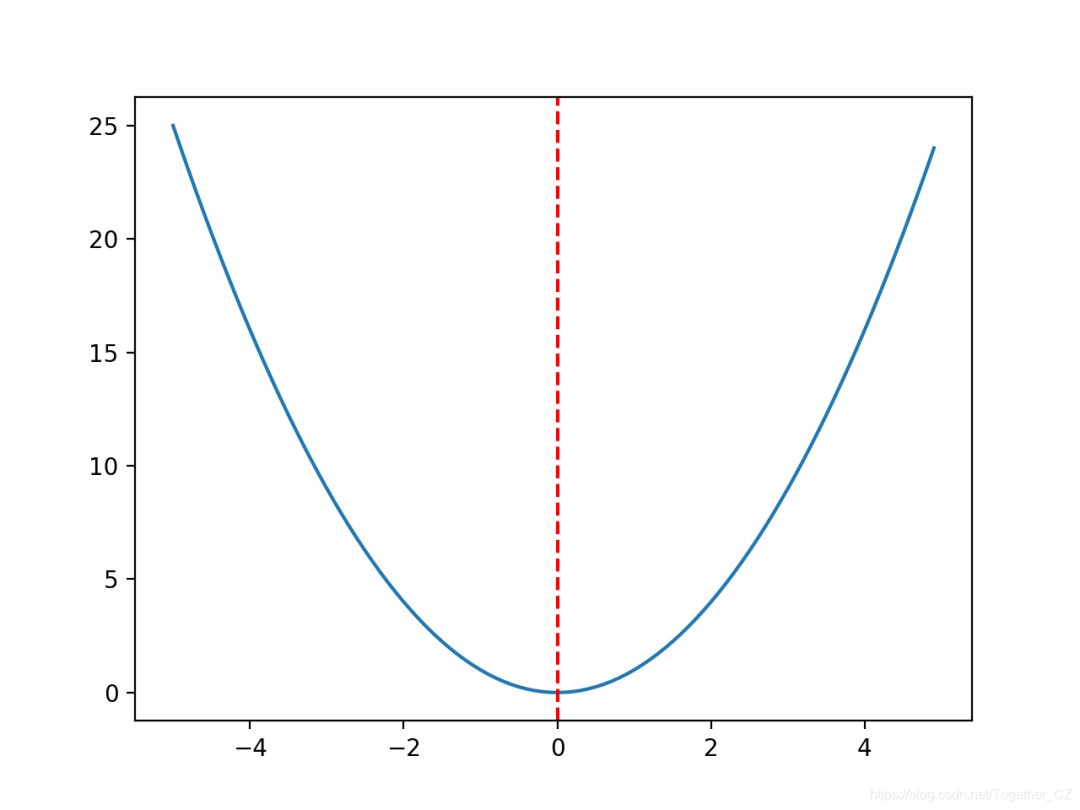
现在，我们知道了如何在Python中实现爬山算法，让我们看看如何使用它来优化目标函数。

应用爬山算法的示例

在本节中，我们将把爬山优化算法应用于目标函数。首先，让我们定义目标函数。我们将使用一个简单的一维x ^ 2目标函数，其边界为[-5，5]。下面的示例定义了函数，然后为输入值的网格创建了函数响应面的折线图，并用红线标记了f（0.0）= 0.0处的最佳值。

# convex unimodal optimization function
from numpy import arange
from matplotlib import pyplot
 
# objective function
def objective(x):
 return x[0]**2.0
 
# define range for input
r_min, r_max = -5.0, 5.0
# sample input range uniformly at 0.1 increments
inputs = arange(r_min, r_max, 0.1)
# compute targets
results = [objective([x]) for x in inputs]
# create a line plot of input vs result
pyplot.plot(inputs, results)
# define optimal input value
x_optima = 0.0
# draw a vertical line at the optimal input
pyplot.axvline(x=x_optima, ls='--', color='red')
# show the plot
pyplot.show()

运行示例将创建目标函数的折线图，并清晰地标记函数的最优值。

接下来，我们可以将爬山算法应用于目标函数。首先，我们将播种伪随机数生成器。通常这不是必需的，但是在这种情况下，我想确保每次运行算法时都得到相同的结果（相同的随机数序列），以便以后可以绘制结果。

# seed the pseudorandom number generator
seed(5)

接下来，我们可以定义搜索的配置。在这种情况下，我们将搜索算法的1,000次迭代，并使用0.1的步长。假设我们使用的是高斯函数来生成步长，这意味着大约99％的所有步长将位于给定点（0.1 * 3）的距离内，例如三个标准差。

n_iterations = 1000
# define the maximum step size
step_size = 0.1

接下来，我们可以执行搜索并报告结果。

# perform the hill climbing search
best, score = hillclimbing(objective, bounds, n_iterations, step_size)
print('Done!')
print('f(%s) = %f' % (best, score))

结合在一起，下面列出了完整的示例。

# hill climbing search of a one-dimensional objective function
from numpy import asarray
from numpy.random import randn
from numpy.random import rand
from numpy.random import seed
 
# objective function
def objective(x):
 return x[0]**2.0
 
# hill climbing local search algorithm
def hillclimbing(objective, bounds, n_iterations, step_size):
 # generate an initial point
 solution = bounds[:, 0] + rand(len(bounds)) * (bounds[:, 1] - bounds[:, 0])
 # evaluate the initial point
 solution_eval = objective(solution)
 # run the hill climb
 for i in range(n_iterations):
  # take a step
  candidate = solution + randn(len(bounds)) * step_size
  # evaluate candidate point
  candidte_eval = objective(candidate)
  # check if we should keep the new point
  if candidte_eval <= solution_eval:
   # store the new point
   solution, solution_eval = candidate, candidte_eval
   # report progress
   print('>%d f(%s) = %.5f' % (i, solution, solution_eval))
 return [solution, solution_eval]
 
# seed the pseudorandom number generator
seed(5)
# define range for input
bounds = asarray([[-5.0, 5.0]])
# define the total iterations
n_iterations = 1000
# define the maximum step size
step_size = 0.1
# perform the hill climbing search
best, score = hillclimbing(objective, bounds, n_iterations, step_size)
print('Done!')
print('f(%s) = %f' % (best, score))

运行该示例将报告搜索进度，包括每次检测到改进时的迭代次数，该函数的输入以及来自目标函数的响应。搜索结束时，找到最佳解决方案，并报告其评估结果。在这种情况下，我们可以看到在算法的1,000次迭代中有36处改进，并且该解决方案非常接近于0.0的最佳输入，其计算结果为f（0.0）= 0.0。

>1 f([-2.74290923]) = 7.52355
>3 f([-2.65873147]) = 7.06885
>4 f([-2.52197291]) = 6.36035
>5 f([-2.46450214]) = 6.07377
>7 f([-2.44740961]) = 5.98981
>9 f([-2.28364676]) = 5.21504
>12 f([-2.19245939]) = 4.80688
>14 f([-2.01001538]) = 4.04016
>15 f([-1.86425287]) = 3.47544
>22 f([-1.79913002]) = 3.23687
>24 f([-1.57525573]) = 2.48143
>25 f([-1.55047719]) = 2.40398
>26 f([-1.51783757]) = 2.30383
>27 f([-1.49118756]) = 2.22364
>28 f([-1.45344116]) = 2.11249
>30 f([-1.33055275]) = 1.77037
>32 f([-1.17805016]) = 1.38780
>33 f([-1.15189314]) = 1.32686
>36 f([-1.03852644]) = 1.07854
>37 f([-0.99135322]) = 0.98278
>38 f([-0.79448984]) = 0.63121
>39 f([-0.69837955]) = 0.48773
>42 f([-0.69317313]) = 0.48049
>46 f([-0.61801423]) = 0.38194
>48 f([-0.48799625]) = 0.23814
>50 f([-0.22149135]) = 0.04906
>54 f([-0.20017144]) = 0.04007
>57 f([-0.15994446]) = 0.02558
>60 f([-0.15492485]) = 0.02400
>61 f([-0.03572481]) = 0.00128
>64 f([-0.03051261]) = 0.00093
>66 f([-0.0074283]) = 0.00006
>78 f([-0.00202357]) = 0.00000
>119 f([0.00128373]) = 0.00000
>120 f([-0.00040911]) = 0.00000
>314 f([-0.00017051]) = 0.00000
Done!
f([-0.00017051]) = 0.000000

以线图的形式查看搜索的进度可能很有趣，该线图显示了每次改进后最佳解决方案的评估变化。每当有改进时，我们就可以更新hillclimbing（）来跟踪目标函数的评估，并返回此分数列表。

# hill climbing local search algorithm
def hillclimbing(objective, bounds, n_iterations, step_size):
 # generate an initial point
 solution = bounds[:, 0] + rand(len(bounds)) * (bounds[:, 1] - bounds[:, 0])
 # evaluate the initial point
 solution_eval = objective(solution)
 # run the hill climb
 scores = list()
 scores.append(solution_eval)
 for i in range(n_iterations):
  # take a step
  candidate = solution + randn(len(bounds)) * step_size
  # evaluate candidate point
  candidte_eval = objective(candidate)
  # check if we should keep the new point
  if candidte_eval <= solution_eval:
   # store the new point
   solution, solution_eval = candidate, candidte_eval
   # keep track of scores
   scores.append(solution_eval)
   # report progress
   print('>%d f(%s) = %.5f' % (i, solution, solution_eval))
 return [solution, solution_eval, scores]

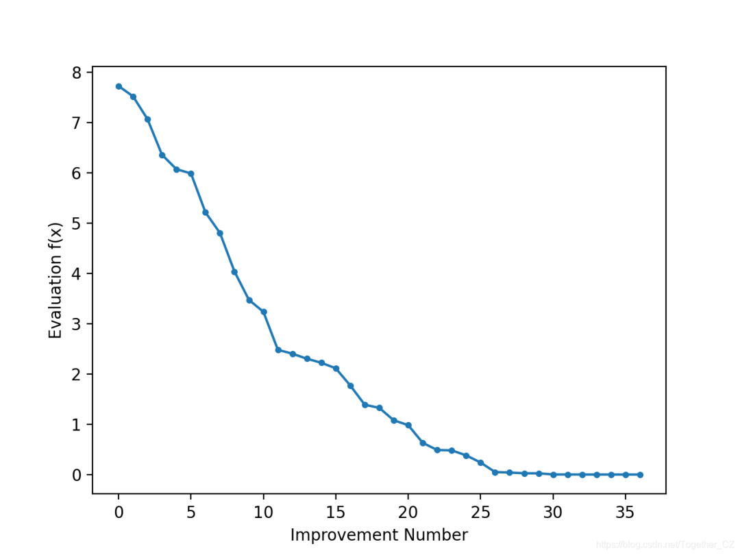
然后，我们可以创建这些分数的折线图，以查看搜索过程中发现的每个改进的目标函数的相对变化。

# line plot of best scores
pyplot.plot(scores, '.-')
pyplot.xlabel('Improvement Number')
pyplot.ylabel('Evaluation f(x)')
pyplot.show()

结合在一起，下面列出了执行搜索并绘制搜索过程中改进解决方案的目标函数得分的完整示例。

# hill climbing search of a one-dimensional objective function
from numpy import asarray
from numpy.random import randn
from numpy.random import rand
from numpy.random import seed
from matplotlib import pyplot
 
# objective function
def objective(x):
 return x[0]**2.0
 
# hill climbing local search algorithm
def hillclimbing(objective, bounds, n_iterations, step_size):
 # generate an initial point
 solution = bounds[:, 0] + rand(len(bounds)) * (bounds[:, 1] - bounds[:, 0])
 # evaluate the initial point
 solution_eval = objective(solution)
 # run the hill climb
 scores = list()
 scores.append(solution_eval)
 for i in range(n_iterations):
  # take a step
  candidate = solution + randn(len(bounds)) * step_size
  # evaluate candidate point
  candidte_eval = objective(candidate)
  # check if we should keep the new point
  if candidte_eval <= solution_eval:
   # store the new point
   solution, solution_eval = candidate, candidte_eval
   # keep track of scores
   scores.append(solution_eval)
   # report progress
   print('>%d f(%s) = %.5f' % (i, solution, solution_eval))
 return [solution, solution_eval, scores]
 
# seed the pseudorandom number generator
seed(5)
# define range for input
bounds = asarray([[-5.0, 5.0]])
# define the total iterations
n_iterations = 1000
# define the maximum step size
step_size = 0.1
# perform the hill climbing search
best, score, scores = hillclimbing(objective, bounds, n_iterations, step_size)
print('Done!')
print('f(%s) = %f' % (best, score))
# line plot of best scores
pyplot.plot(scores, '.-')
pyplot.xlabel('Improvement Number')
pyplot.ylabel('Evaluation f(x)')
pyplot.show()

运行示例将执行搜索，并像以前一样报告结果。创建一个线形图，显示在爬山搜索期间每个改进的目标函数评估。在搜索过程中，我们可以看到目标函数评估发生了约36个变化，随着算法收敛到最优值，初始变化较大，而在搜索结束时变化很小，难以察觉。

鉴于目标函数是一维的，因此可以像上面那样直接绘制响应面。通过将在搜索过程中找到的最佳候选解决方案绘制为响应面中的点，来回顾搜索的进度可能会很有趣。我们期望沿着响应面到达最优点的一系列点。这可以通过首先更新hillclimbing（）函数以跟踪每个最佳候选解决方案在搜索过程中的位置来实现，然后返回最佳解决方案列表来实现。

# hill climbing local search algorithm
def hillclimbing(objective, bounds, n_iterations, step_size):
 # generate an initial point
 solution = bounds[:, 0] + rand(len(bounds)) * (bounds[:, 1] - bounds[:, 0])
 # evaluate the initial point
 solution_eval = objective(solution)
 # run the hill climb
 solutions = list()
 solutions.append(solution)
 for i in range(n_iterations):
  # take a step
  candidate = solution + randn(len(bounds)) * step_size
  # evaluate candidate point
  candidte_eval = objective(candidate)
  # check if we should keep the new point
  if candidte_eval <= solution_eval:
   # store the new point
   solution, solution_eval = candidate, candidte_eval
   # keep track of solutions
   solutions.append(solution)
   # report progress
   print('>%d f(%s) = %.5f' % (i, solution, solution_eval))
 return [solution, solution_eval, solutions]

然后，我们可以创建目标函数响应面的图，并像以前那样标记最优值。

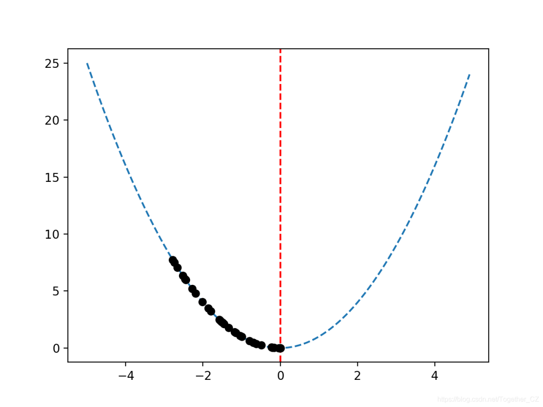
# sample input range uniformly at 0.1 increments
inputs = arange(bounds[0,0], bounds[0,1], 0.1)
# create a line plot of input vs result
pyplot.plot(inputs, [objective([x]) for x in inputs], '--')
# draw a vertical line at the optimal input
pyplot.axvline(x=[0.0], ls='--', color='red')

最后，我们可以将搜索找到的候选解的序列绘制成黑点。

# plot the sample as black circles
pyplot.plot(solutions, [objective(x) for x in solutions], 'o', color='black')

结合在一起，下面列出了在目标函数的响应面上绘制改进解序列的完整示例。

# hill climbing search of a one-dimensional objective function
from numpy import asarray
from numpy import arange
from numpy.random import randn
from numpy.random import rand
from numpy.random import seed
from matplotlib import pyplot
 
# objective function
def objective(x):
 return x[0]**2.0
 
# hill climbing local search algorithm
def hillclimbing(objective, bounds, n_iterations, step_size):
 # generate an initial point
 solution = bounds[:, 0] + rand(len(bounds)) * (bounds[:, 1] - bounds[:, 0])
 # evaluate the initial point
 solution_eval = objective(solution)
 # run the hill climb
 solutions = list()
 solutions.append(solution)
 for i in range(n_iterations):
  # take a step
  candidate = solution + randn(len(bounds)) * step_size
  # evaluate candidate point
  candidte_eval = objective(candidate)
  # check if we should keep the new point
  if candidte_eval <= solution_eval:
   # store the new point
   solution, solution_eval = candidate, candidte_eval
   # keep track of solutions
   solutions.append(solution)
   # report progress
   print('>%d f(%s) = %.5f' % (i, solution, solution_eval))
 return [solution, solution_eval, solutions]
 
# seed the pseudorandom number generator
seed(5)
# define range for input
bounds = asarray([[-5.0, 5.0]])
# define the total iterations
n_iterations = 1000
# define the maximum step size
step_size = 0.1
# perform the hill climbing search
best, score, solutions = hillclimbing(objective, bounds, n_iterations, step_size)
print('Done!')
print('f(%s) = %f' % (best, score))
# sample input range uniformly at 0.1 increments
inputs = arange(bounds[0,0], bounds[0,1], 0.1)
# create a line plot of input vs result
pyplot.plot(inputs, [objective([x]) for x in inputs], '--')
# draw a vertical line at the optimal input
pyplot.axvline(x=[0.0], ls='--', color='red')
# plot the sample as black circles
pyplot.plot(solutions, [objective(x) for x in solutions], 'o', color='black')
pyplot.show()

运行示例将执行爬山搜索，并像以前一样报告结果。像以前一样创建一个响应面图，显示函数的熟悉的碗形，并用垂直的红线标记函数的最佳状态。在搜索过程中找到的最佳解决方案的顺序显示为黑点，沿着碗形延伸到最佳状态。

作者：沂水寒城，CSDN博客专家，个人研究方向：机器学习、深度学习、NLP、CV

Blog: http://yishuihancheng.blog.csdn.net

赞赏作者

更多阅读

2020 年最佳流行 Python 库 Top 10

2020 Python中文社区热门文章 Top 10

5分钟快速掌握 Python 定时任务框架

特别推荐

点击下方阅读原文加入社区会员