
(附代码解析)目标检测比赛中的tricks集锦
点击左上方蓝字关注我们

转载自 | 极市平台
作者 | 初识CV@知乎
链接 | https://zhuanlan.zhihu.com/p/102817180
1.数据增强
可参考:
初识CV:MMDetection中文文档
https://zhuanlan.zhihu.com/p/101222759
数据增强是增加深度模型鲁棒性和泛化性能的常用手段,随机翻转、随机裁剪、添加噪声等也被引入到检测任务的训练中来,个人认为数据(监督信息)的适时传入可能是更有潜力的方向。
个人观点:
问题: 为什么图像和Bbox需要进行数据增强呢?
答: 因为数据多了就可以尽可能多的学习到图像中的不变性,学习到的不变性越多那么模型的泛化能力越强。
但是输入到CNN中的图像为什么不具有平移不变性?如何去解决?下面链接有专门的解析:
初识CV:输入到CNN中的图像为什么不具有平移不变性?如何去解决?
https://zhuanlan.zhihu.com/p/103342289
MMDetection中,数据增强包括两部分:(源码解析)
新版MMDetection新添加用Albu数据库对图像进行增强的代码,位置在mmdetection/configs/albu_example/mask_rcnn_r50_fpn_1x.py,是基于图像分割的,用于目标检测的代码更新如下:
初识CV:目标检测tricks:Ablu数据库增强
https://zhuanlan.zhihu.com/p/125036517
图像增强。
1.1 引入albumentations数据增强库进行增强
这部分代码需要看开头‘注意’部分解析,防止修改代码后运行报错。
需要修改两个部分代码:
mmdet/datasets/pipelines/transforms.py,修改后的源码如下:
mmdet/datasets/pipelines/transforms.py
https://zhuanlan.zhihu.com/p/107922611
mmdet/datasets/pipelines/__init__.py,修改后的源码如下:
mmdet/datasets/pipelines/__init__.py
https://zhuanlan.zhihu.com/p/107922962
具体修改方式如下:添加dict(type='Albu', transforms = [{"type": 'RandomRotate90'}]),其他的类似。
train_pipeline = [dict(type='LoadImageFromFile'),dict(type='LoadAnnotations', with_bbox=True),dict(type='Albu', transforms = [{"type": 'RandomRotate90'}]),# 数据增强dict(type='Resize', img_scale=(1333, 800), keep_ratio=True),dict(type='RandomFlip', flip_ratio=0.5),dict(type='Normalize', **img_norm_cfg),dict(type='Pad', size_divisor=32),dict(type='DefaultFormatBundle'),dict(type='Collect', keys=['img', 'gt_bboxes', 'gt_labels']),]
1.2 MMDetection自带数据增强:
源码在mmdet/datasets/extra_aug.py里面,包括RandomCrop、brightness、contrast、saturation、ExtraAugmentation等等图像增强方法。 添加位置是train_pipeline或test_pipeline这个地方(一般train进行增强而test不需要),例如数据增强RandomFlip,flip_ratio代表随机翻转的概率:
train_pipeline = [dict(type='LoadImageFromFile'),dict(type='LoadAnnotations', with_bbox=True),dict(type='Resize', img_scale=(1333, 800), keep_ratio=True),dict(type='RandomFlip', flip_ratio=0.5),dict(type='Normalize', **img_norm_cfg),dict(type='Pad', size_divisor=32),dict(type='DefaultFormatBundle'),dict(type='Collect', keys=['img', 'gt_bboxes', 'gt_labels']),]test_pipeline = [dict(type='LoadImageFromFile'),dict(type='MultiScaleFlipAug',img_scale=(1333, 800),flip=False,transforms=[dict(type='Resize', keep_ratio=True),dict(type='RandomFlip'),dict(type='Normalize', **img_norm_cfg),dict(type='Pad', size_divisor=32),dict(type='ImageToTensor', keys=['img']),dict(type='Collect', keys=['img']),])]
2. Bbox增强
albumentations数据增强(同上) 源码在mmdet/datasets/custom.py里面,增强源码为:
def pre_pipeline(self, results):results['img_prefix'] = self.img_prefixresults['seg_prefix'] = self.seg_prefixresults['proposal_file'] = self.proposal_fileresults['bbox_fields'] = []results['mask_fields'] = []
2.Multi-scale Training/Testing 多尺度训练/测试
可参考:
初识CV:MMDetection中文文档—4.技术细节
https://zhuanlan.zhihu.com/p/101222759
输入图片的尺寸对检测模型的性能影响相当明显,事实上,多尺度是提升精度最明显的技巧之一。在基础网络部分常常会生成比原图小数十倍的特征图,导致小物体的特征描述不容易被检测网络捕捉。通过输入更大、更多尺寸的图片进行训练,能够在一定程度上提高检测模型对物体大小的鲁棒性,仅在测试阶段引入多尺度,也可享受大尺寸和多尺寸带来的增益。
multi-scale training/testing最早见于[1],训练时,预先定义几个固定的尺度,每个epoch随机选择一个尺度进行训练。测试时,生成几个不同尺度的feature map,对每个Region Proposal,在不同的feature map上也有不同的尺度,我们选择最接近某一固定尺寸(即检测头部的输入尺寸)的Region Proposal作为后续的输入。在[2]中,选择单一尺度的方式被Maxout(element-wise max,逐元素取最大)取代:随机选两个相邻尺度,经过Pooling后使用Maxout进行合并,如下图所示。
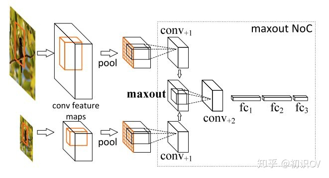
使用Maxout合并feature vector
近期的工作如FPN等已经尝试在不同尺度的特征图上进行检测,但多尺度训练/测试仍作为一种提升性能的有效技巧被应用在MS COCO等比赛中。
问题:多尺度的选择有什么规则和技巧吗?
答:如果模型不考虑时间开销,尺寸往大的开。一般来说尺度越大效果越好,主要是因为检测的小目标越多效果越差。如果是新手那就按照默认参数的比例扩大就行了,然后测试的时候取训练集的中间值。比如cascade50默认尺度是(1333,800),多尺度可以按照默认尺度的倍数扩大比如扩大两倍(2666,1600),多尺度训练可以写成[(1333, 800), (2666, 1600)],单尺度测试可以选择(2000, 1200),多尺度测试可以选择为多尺度训练的尺度加上他们的中间值[(1333, 800), (2000, 1200),(2666, 1600)]。keep_ratio=True,一般不考虑长边。
MMDetection中,多尺度训练/测试:(源码解析)
只需要修改train_pipeline 和test_pipeline中的img_scale部分即可(换成[(), ()]或者[(), (), ().....])。带来的影响是:train达到拟合的时间增加、test的时间增加,一旦test的时间增加一定会影响比赛的分数,因为比赛都会将测试的时间作为评分标准之一:
参数解析:
train_pipeline中dict(type='Resize', img_scale=(1333, 800), keep_ratio=True)的keep_ratio解析。假设原始图像大小为(1500, 1000),ratio=长边/短边 = 1.5。
当keep_ratio=True时,img_scale的多尺度最多为两个。假设多尺度为[(2000, 1200), (1333, 800)],则代表的含义为:首先将图像的短边固定到800到1200范围中的某一个数值假设为1100,那么对应的长边应该是短边的ratio=1.5倍为 ,且长边的取值在1333到2000的范围之内。如果大于2000按照2000计算,小于1300按照1300计算。 当keep_ratio=False时,img_scale的多尺度可以为任意多个。假设多尺度为[(2000, 1200), (1666, 1000),(1333, 800)],则代表的含义为:随机从三个尺度中选取一个作为图像的尺寸进行训练。 test_pipeline 中img_scale的尺度可以为任意多个,含义为对测试集进行多尺度测试(可以理解为TTA)。
train_pipeline = [dict(type='LoadImageFromFile'),dict(type='LoadAnnotations', with_bbox=True),dict(type='Resize', img_scale=(1333, 800), keep_ratio=True), #这里可以更换多尺度[(),()]dict(type='RandomFlip', flip_ratio=0.5),dict(type='Normalize', **img_norm_cfg),dict(type='Pad', size_divisor=32),dict(type='DefaultFormatBundle'),dict(type='Collect', keys=['img', 'gt_bboxes', 'gt_labels']),]test_pipeline = [dict(type='LoadImageFromFile'),dict(type='MultiScaleFlipAug',img_scale=(1333, 800), #这里可以更换多尺度[(),()]flip=False,transforms=[dict(type='Resize', keep_ratio=True),dict(type='RandomFlip'),dict(type='Normalize', **img_norm_cfg),dict(type='Pad', size_divisor=32),dict(type='ImageToTensor', keys=['img']),dict(type='Collect', keys=['img']),])]
3.Global Context 全局语境
这一技巧在ResNet的工作[3]中提出,做法是把整张图片作为一个RoI,对其进行RoI Pooling并将得到的feature vector拼接于每个RoI的feature vector上,作为一种辅助信息传入之后的R-CNN子网络。目前,也有把相邻尺度上的RoI互相作为context共同传入的做法。
这一部分暂时没有代码解析。
4.Box Refinement/Voting 预测框微调/投票法/模型融合
微调法和投票法由工作[4]提出,前者也被称为Iterative Localization。
微调法最初是在SS算法得到的Region Proposal基础上用检测头部进行多次迭代得到一系列box,在ResNet的工作中,作者将输入R-CNN子网络的Region Proposal和R-CNN子网络得到的预测框共同进行NMS(见下面小节)后处理,最后,把跟NMS筛选所得预测框的IoU超过一定阈值的预测框进行按其分数加权的平均,得到最后的预测结果。
投票法可以理解为以顶尖筛选出一流,再用一流的结果进行加权投票决策。
不同的训练策略,不同的 epoch 预测的结果,使用 NMS 来融合,或者soft_nms
需要调整的参数:
box voting 的阈值。 不同的输入中这个框至少出现了几次来允许它输出。 得分的阈值,一个目标框的得分低于这个阈值的时候,就删掉这个目标框。
模型融合主要分为两种情况:
这里主要是在nms之前,对于不同模型预测出来的结果,根据score来排序再做nms操作。
2. 多个模型的融合
这里是指不同的方法,比如说faster rcnn与retinanet的融合,可以有两种情况:
a) 取并集,防止漏检。
b) 取交集,防止误检,提高精度。
5.随机权值平均(Stochastic Weight Averaging,SWA)
随机权值平均只需快速集合集成的一小部分算力,就可以接近其表现。SWA 可以用在任意架构和数据集上,都会有不错的表现。根据论文中的实验,SWA 可以得到我之前提到过的更宽的极小值。在经典认知下,SWA 不算集成,因为在训练的最终阶段你只得到一个模型,但它的表现超过了快照集成,接近 FGE(多个模型取平均)。
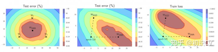
左图:W1、W2、W3分别代表3个独立训练的网络,Wswa为其平均值。中图:WSWA 在测试集上的表现超越了SGD。右图:WSWA 在训练时的损失比SGD要高。
结合 WSWA 在测试集上优于 SGD 的表现,这意味着尽管 WSWA 训练时的损失较高,它的泛化性更好。
SWA 的直觉来自以下由经验得到的观察:每个学习率周期得到的局部极小值倾向于堆积在损失平面的低损失值区域的边缘(上图左侧的图形中,褐色区域误差较低,点W1、W2、3分别表示3个独立训练的网络,位于褐色区域的边缘)。对这些点取平均值,可能得到一个宽阔的泛化解,其损失更低(上图左侧图形中的 WSWA)。
下面是 SWA 的工作原理。它只保存两个模型,而不是许多模型的集成:
第一个模型保存模型权值的平均值(WSWA)。在训练结束后,它将是用于预测的最终模型。 第二个模型(W)将穿过权值空间,基于周期性学习率规划探索权重空间。
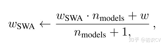
SWA权重更新公式
在每个学习率周期的末尾,第二个模型的当前权重将用来更新第一个模型的权重(公式如上)。因此,在训练阶段,只需训练一个模型,并在内存中储存两个模型。预测时只需要平均模型,基于其进行预测将比之前描述的集成快很多,因为在那种集成中,你需要使用多个模型进行预测,最后再进行平均。
方法实现:
论文的作者自己提供了一份 PyTorch 的实现 :
timgaripov/swa
https://github.com/timgaripov/swa
此外,基于 fast.ai 库的 SWA 可见 :
Add Stochastic Weight Averaging by wdhorton · Pull Request #276 · fastai/fastai
https://github.com/fastai/fastai/pull/276/commits
6.OHEM 在线难例挖掘
OHEM(Online Hard negative Example Mining,https://arxiv.org/pdf/1604.03540.pdf),在线难例挖掘)见于[5]。两阶段检测模型中,提出的RoI Proposal在输入R-CNN子网络前,我们有机会对正负样本(背景类和前景类)的比例进行调整。通常,背景类的RoI Proposal个数要远远多于前景类,Fast R-CNN的处理方式是随机对两种样本进行上采样和下采样,以使每一batch的正负样本比例保持在1:3,这一做法缓解了类别比例不均衡的问题,是两阶段方法相比单阶段方法具有优势的地方,也被后来的大多数工作沿用。
论文中把OHEM应用在Fast R-CNN,是因为Fast R-CNN相当于目标检测各大框架的母体,很多框架都是它的变形,所以作者在Fast R-CNN上应用很有说明性。
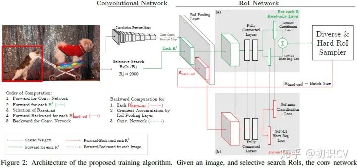
Fast R-CNN框架
上图是Fast R-CNN框架,简单的说,Fast R-CNN框架是将224×224的图片当作输入,经过conv,pooling等操作输出feature map,通过selective search 创建2000个region proposal,将其一起输入ROI pooling层,接上全连接层与两个损失层。
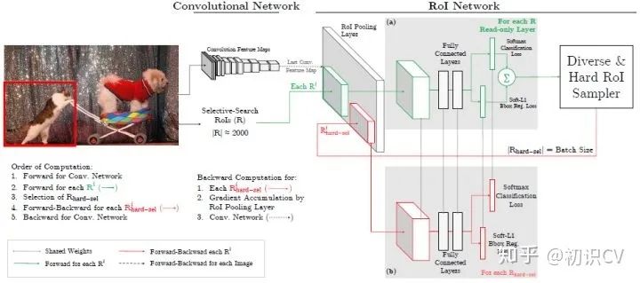
OHEM图解,应用于Fast R-CNN
作者将OHEM应用在Fast R-CNN的网络结构,如上图,这里包含两个RoI network,上面一个RoI network是只读的,为所有的RoI 在前向传递的时候分配空间,下面一个RoI network则同时为前向和后向分配空间。在OHEM的工作中,作者提出用R-CNN子网络对RoI Proposal预测的分数来决定每个batch选用的样本。这样,输入R-CNN子网络的RoI Proposal总为其表现不好的样本,提高了监督学习的效率。
首先,RoI 经过RoI plooling层生成feature map,然后进入只读的RoI network得到所有RoI 的loss;然后是hard RoI sampler结构根据损失排序选出hard example,并把这些hard example作为下面那个RoI network的输入。
实际训练的时候,每个mini-batch包含N个图像,共|R|个RoI ,也就是每张图像包含|R|/N个RoI 。经过hard RoI sampler筛选后得到B个hard example。作者在文中采用N=2,|R|=4000,B=128。另外关于正负样本的选择:当一个RoI 和一个ground truth的IoU大于0.5,则为正样本;当一个RoI 和所有ground truth的IoU的最大值小于0.5时为负样本。
总结来说,对于给定图像,经过selective search RoIs,同样计算出卷积特征图。但是在绿色部分的(a)中,一个只读的RoI网络对特征图和所有RoI进行前向传播,然后Hard RoI module利用这些RoI的loss选择B个样本。在红色部分(b)中,这些选择出的样本(hard examples)进入RoI网络,进一步进行前向和后向传播。
MMDetection中,OHEM(online hard example mining):(源码解析)
rcnn=[dict(assigner=dict(type='MaxIoUAssigner',pos_iou_thr=0.4, # 更换neg_iou_thr=0.4,min_pos_iou=0.4,ignore_iof_thr=-1),sampler=dict(type='OHEMSampler',num=512,pos_fraction=0.25,neg_pos_ub=-1,add_gt_as_proposals=True),pos_weight=-1,debug=False),dict(assigner=dict(type='MaxIoUAssigner',pos_iou_thr=0.5,neg_iou_thr=0.5,min_pos_iou=0.5,ignore_iof_thr=-1),sampler=dict(type='OHEMSampler', # 解决难易样本,也解决了正负样本比例问题。num=512,pos_fraction=0.25,neg_pos_ub=-1,add_gt_as_proposals=True),pos_weight=-1,debug=False),dict(assigner=dict(type='MaxIoUAssigner',pos_iou_thr=0.6,neg_iou_thr=0.6,min_pos_iou=0.6,ignore_iof_thr=-1),sampler=dict(type='OHEMSampler',num=512,pos_fraction=0.25,neg_pos_ub=-1,add_gt_as_proposals=True),pos_weight=-1,debug=False)],stage_loss_weights=[1, 0.5, 0.25])
7.Soft NMS 软化非极大抑制
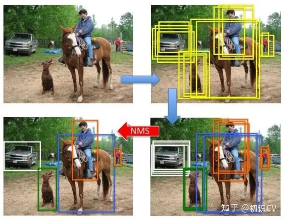
NMS后处理图示
NMS(Non-Maximum Suppression,非极大抑制)是检测模型的标准后处理操作,用于去除重合度(IoU)较高的预测框,只保留预测分数最高的预测框作为检测输出。Soft NMS由[6]提出。在传统的NMS中,跟最高预测分数预测框重合度超出一定阈值的预测框会被直接舍弃,作者认为这样不利于相邻物体的检测。提出的改进方法是根据IoU将预测框的预测分数进行惩罚,最后再按分数过滤。配合Deformable Convnets(将在之后的文章介绍),Soft NMS在MS COCO上取得了当时最佳的表现。算法改进如下:
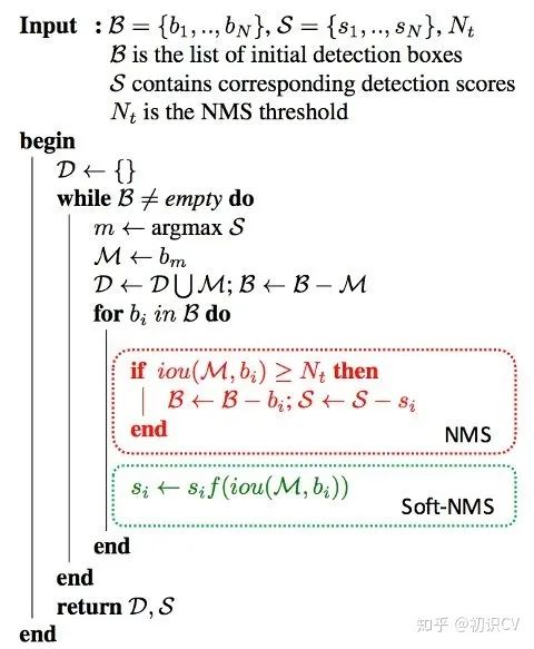
Soft-NMS算法改进
上图中的即为软化函数,通常取线性或高斯函数,后者效果稍好一些。当然,在享受这一增益的同时,Soft-NMS也引入了一些超参,对不同的数据集需要试探以确定最佳配置。
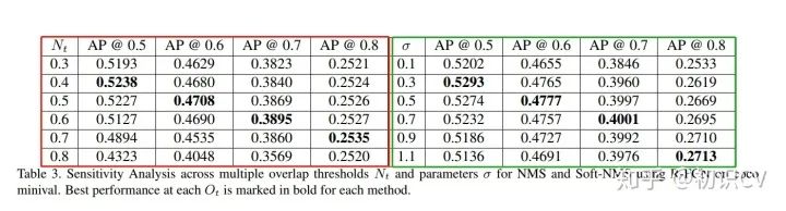
解析Soft NMS论文的一个小知识点:Improving Object Detection With One Line of Code
https://arxiv.org/pdf/1704.04503.pdf
可以根据论文Table3中对应AP@(置信度阈值)的 值设置iou_thr(nms)的值:
左边一半(红色框)是NMS,右边一半(绿色框)是Soft NMS。在NMS部分,相同 (置信度阈值)条件下(较小的情况下),基本上 值越大,其AP值越小。这主要是因为值越大,有越多的重复框没有过滤掉。
左边一半(红色框)是NMS,右边一半(绿色框)是Soft NMS。
MMDetection中,Soft NMS 软化非极大抑制:(源码解析)
test_cfg = dict(rpn=dict(nms_across_levels=False,nms_pre=1000,nms_post=1000,max_num=1000,nms_thr=0.7,min_bbox_size=0),rcnn=dict(score_thr=0.05, nms=dict(type='nms', iou_thr=0.5), max_per_img=100) # max_per_img表示最终输出的det bbox数量# soft-nms is also supported for rcnn testing# e.g., nms=dict(type='soft_nms', iou_thr=0.5, min_score=0.001) # soft_nms参数)
8.RoIAlign RoI对齐
RoIAlign是Mask R-CNN([7])的工作中提出的,针对的问题是RoI在进行Pooling时有不同程度的取整,这影响了实例分割中mask损失的计算。文章采用双线性插值的方法将RoI的表示精细化,并带来了较为明显的性能提升。这一技巧也被后来的一些工作(如light-head R-CNN)沿用。
这一部分暂时没有代码解析。
9.其他方法
除去上面所列的技巧外,还有一些做法也值得注意:
更好的先验(YOLOv2):使用聚类方法统计数据中box标注的大小和长宽比,以更好的设置anchor box的生成配置 更好的pre-train模型:检测模型的基础网络通常使用ImageNet(通常是ImageNet-1k)上训练好的模型进行初始化,使用更大的数据集(ImageNet-5k)预训练基础网络对精度的提升亦有帮助 超参数的调整:部分工作也发现如NMS中IoU阈值的调整(从0.3到0.5)也有利于精度的提升,但这一方面尚无最佳配置参照
最后,集成(Ensemble)作为通用的手段也被应用在比赛中。
代码部分
1.各部分代码解析
1.1 faster_rcnn_r50_fpn_1x.py:
首先介绍一下这个配置文件所描述的框架,它是基于resnet50的backbone,有着5个fpn特征层的faster-RCNN目标检测网络,训练迭代次数为标准的12次epoch。
# model settingsmodel = dict(type='FasterRCNN', # model类型pretrained='modelzoo://resnet50', # 预训练模型:imagenet-resnet50backbone=dict(type='ResNet', # backbone类型depth=50, # 网络层数num_stages=4, # resnet的stage数量out_indices=(0, 1, 2, 3), # 输出的stage的序号frozen_stages=1, # 冻结的stage数量,即该stage不更新参数,-1表示所有的stage都更新参数style='pytorch'), # 网络风格:如果设置pytorch,则stride为2的层是conv3x3的卷积层;如果设置caffe,则stride为2的层是第一个conv1x1的卷积层neck=dict(type='FPN', # neck类型in_channels=[256, 512, 1024, 2048], # 输入的各个stage的通道数out_channels=256, # 输出的特征层的通道数num_outs=5), # 输出的特征层的数量rpn_head=dict(type='RPNHead', # RPN网络类型in_channels=256, # RPN网络的输入通道数feat_channels=256, # 特征层的通道数anchor_scales=[8], # 生成的anchor的baselen,baselen = sqrt(w*h),w和h为anchor的宽和高anchor_ratios=[0.5, 1.0, 2.0], # anchor的宽高比anchor_strides=[4, 8, 16, 32, 64], # 在每个特征层上的anchor的步长(对应于原图)target_means=[.0, .0, .0, .0], # 均值target_stds=[1.0, 1.0, 1.0, 1.0], # 方差use_sigmoid_cls=True), # 是否使用sigmoid来进行分类,如果False则使用softmax来分类bbox_roi_extractor=dict(type='SingleRoIExtractor', # RoIExtractor类型roi_layer=dict(type='RoIAlign', out_size=7, sample_num=2), # ROI具体参数:ROI类型为ROIalign,输出尺寸为7,sample数为2out_channels=256, # 输出通道数featmap_strides=[4, 8, 16, 32]), # 特征图的步长bbox_head=dict(type='SharedFCBBoxHead', # 全连接层类型num_fcs=2, # 全连接层数量in_channels=256, # 输入通道数fc_out_channels=1024, # 输出通道数roi_feat_size=7, # ROI特征层尺寸num_classes=81, # 分类器的类别数量+1,+1是因为多了一个背景的类别target_means=[0., 0., 0., 0.], # 均值target_stds=[0.1, 0.1, 0.2, 0.2], # 方差reg_class_agnostic=False)) # 是否采用class_agnostic的方式来预测,class_agnostic表示输出bbox时只考虑其是否为前景,后续分类的时候再根据该bbox在网络中的类别得分来分类,也就是说一个框可以对应多个类别# model training and testing settingstrain_cfg = dict(rpn=dict(assigner=dict(type='MaxIoUAssigner', # RPN网络的正负样本划分pos_iou_thr=0.7, # 正样本的iou阈值neg_iou_thr=0.3, # 负样本的iou阈值min_pos_iou=0.3, # 正样本的iou最小值。如果assign给ground truth的anchors中最大的IOU低于0.3,则忽略所有的anchors,否则保留最大IOU的anchorignore_iof_thr=-1), # 忽略bbox的阈值,当ground truth中包含需要忽略的bbox时使用,-1表示不忽略sampler=dict(type='RandomSampler', # 正负样本提取器类型num=256, # 需提取的正负样本数量pos_fraction=0.5, # 正样本比例neg_pos_ub=-1, # 最大负样本比例,大于该比例的负样本忽略,-1表示不忽略add_gt_as_proposals=False), # 把ground truth加入proposal作为正样本allowed_border=0, # 允许在bbox周围外扩一定的像素pos_weight=-1, # 正样本权重,-1表示不改变原始的权重smoothl1_beta=1 / 9.0, # 平滑L1系数debug=False), # debug模式rcnn=dict(assigner=dict(type='MaxIoUAssigner', # RCNN网络正负样本划分pos_iou_thr=0.5, # 正样本的iou阈值neg_iou_thr=0.5, # 负样本的iou阈值min_pos_iou=0.5, # 正样本的iou最小值。如果assign给ground truth的anchors中最大的IOU低于0.3,则忽略所有的anchors,否则保留最大IOU的anchorignore_iof_thr=-1), # 忽略bbox的阈值,当ground truth中包含需要忽略的bbox时使用,-1表示不忽略sampler=dict(type='RandomSampler', # 正负样本提取器类型num=512, # 需提取的正负样本数量pos_fraction=0.25, # 正样本比例neg_pos_ub=-1, # 最大负样本比例,大于该比例的负样本忽略,-1表示不忽略add_gt_as_proposals=True), # 把ground truth加入proposal作为正样本pos_weight=-1, # 正样本权重,-1表示不改变原始的权重debug=False)) # debug模式test_cfg = dict(rpn=dict( # 推断时的RPN参数nms_across_levels=False, # 在所有的fpn层内做nmsnms_pre=2000, # 在nms之前保留的的得分最高的proposal数量nms_post=2000, # 在nms之后保留的的得分最高的proposal数量max_num=2000, # 在后处理完成之后保留的proposal数量nms_thr=0.7, # nms阈值min_bbox_size=0), # 最小bbox尺寸rcnn=dict(score_thr=0.05, nms=dict(type='nms', iou_thr=0.5), max_per_img=100) # max_per_img表示最终输出的det bbox数量# soft-nms is also supported for rcnn testing# e.g., nms=dict(type='soft_nms', iou_thr=0.5, min_score=0.05) # soft_nms参数)# dataset settingsdataset_type = 'CocoDataset' # 数据集类型data_root = 'data/coco/' # 数据集根目录img_norm_cfg = dict(mean=[123.675, 116.28, 103.53], std=[58.395, 57.12, 57.375], to_rgb=True) # 输入图像初始化,减去均值mean并处以方差std,to_rgb表示将bgr转为rgbdata = dict(imgs_per_gpu=2, # 每个gpu计算的图像数量workers_per_gpu=2, # 每个gpu分配的线程数train=dict(type=dataset_type, # 数据集类型ann_file=data_root + 'annotations/instances_train2017.json', # 数据集annotation路径img_prefix=data_root + 'train2017/', # 数据集的图片路径img_scale=(1333, 800), # 输入图像尺寸,最大边1333,最小边800img_norm_cfg=img_norm_cfg, # 图像初始化参数size_divisor=32, # 对图像进行resize时的最小单位,32表示所有的图像都会被resize成32的倍数flip_ratio=0.5, # 图像的随机左右翻转的概率with_mask=False, # 训练时附带maskwith_crowd=True, # 训练时附带difficult的样本with_label=True), # 训练时附带labelval=dict(type=dataset_type, # 同上ann_file=data_root + 'annotations/instances_val2017.json', # 同上img_prefix=data_root + 'val2017/', # 同上img_scale=(1333, 800), # 同上img_norm_cfg=img_norm_cfg, # 同上size_divisor=32, # 同上flip_ratio=0, # 同上with_mask=False, # 同上with_crowd=True, # 同上with_label=True), # 同上test=dict(type=dataset_type, # 同上ann_file=data_root + 'annotations/instances_val2017.json', # 同上img_prefix=data_root + 'val2017/', # 同上img_scale=(1333, 800), # 同上img_norm_cfg=img_norm_cfg, # 同上size_divisor=32, # 同上flip_ratio=0, # 同上with_mask=False, # 同上with_label=False, # 同上test_mode=True)) # 同上# optimizeroptimizer = dict(type='SGD', lr=0.02, momentum=0.9, weight_decay=0.0001) # 优化参数,lr为学习率,momentum为动量因子,weight_decay为权重衰减因子optimizer_config = dict(grad_clip=dict(max_norm=35, norm_type=2)) # 梯度均衡参数# learning policylr_config = dict(policy='step', # 优化策略warmup='linear', # 初始的学习率增加的策略,linear为线性增加warmup_iters=500, # 在初始的500次迭代中学习率逐渐增加warmup_ratio=1.0 / 3, # 起始的学习率step=[8, 11]) # 在第8和11个epoch时降低学习率checkpoint_config = dict(interval=1) # 每1个epoch存储一次模型# yapf:disablelog_config = dict(interval=50, # 每50个batch输出一次信息hooks=[dict(type='TextLoggerHook'), # 控制台输出信息的风格# dict(type='TensorboardLoggerHook')])# yapf:enable# runtime settingstotal_epochs = 12 # 最大epoch数dist_params = dict(backend='nccl') # 分布式参数log_level = 'INFO' # 输出信息的完整度级别work_dir = './work_dirs/faster_rcnn_r50_fpn_1x' # log文件和模型文件存储路径load_from = None # 加载模型的路径,None表示从预训练模型加载resume_from = None # 恢复训练模型的路径workflow = [('train', 1)] # 当前工作区名称
1.2 cascade_rcnn_r50_fpn_1x.py
cascade-RCNN是cvpr2018的文章,相比于faster-RCNN的改进主要在于其RCNN有三个stage,这三个stage逐级refine检测的结果,使得结果达到更高的精度。下面逐条解释其config的含义,与faster-RCNN相同的部分就不再赘述
# model settingsmodel = dict(type='CascadeRCNN',num_stages=3, # RCNN网络的stage数量,在faster-RCNN中为1pretrained='modelzoo://resnet50',backbone=dict(type='ResNet',depth=50,num_stages=4,out_indices=(0, 1, 2, 3),frozen_stages=1,style='pytorch'),neck=dict(type='FPN',in_channels=[256, 512, 1024, 2048],out_channels=256,num_outs=5),rpn_head=dict(type='RPNHead',in_channels=256,feat_channels=256,anchor_scales=[8],anchor_ratios=[0.5, 1.0, 2.0],anchor_strides=[4, 8, 16, 32, 64],target_means=[.0, .0, .0, .0],target_stds=[1.0, 1.0, 1.0, 1.0],use_sigmoid_cls=True),bbox_roi_extractor=dict(type='SingleRoIExtractor',roi_layer=dict(type='RoIAlign', out_size=7, sample_num=2),out_channels=256,featmap_strides=[4, 8, 16, 32]),bbox_head=[dict(type='SharedFCBBoxHead',num_fcs=2,in_channels=256,fc_out_channels=1024,roi_feat_size=7,num_classes=81,target_means=[0., 0., 0., 0.],target_stds=[0.1, 0.1, 0.2, 0.2],reg_class_agnostic=True),dict(type='SharedFCBBoxHead',num_fcs=2,in_channels=256,fc_out_channels=1024,roi_feat_size=7,num_classes=81,target_means=[0., 0., 0., 0.],target_stds=[0.05, 0.05, 0.1, 0.1],reg_class_agnostic=True),dict(type='SharedFCBBoxHead',num_fcs=2,in_channels=256,fc_out_channels=1024,roi_feat_size=7,num_classes=81,target_means=[0., 0., 0., 0.],target_stds=[0.033, 0.033, 0.067, 0.067],reg_class_agnostic=True)])# model training and testing settingstrain_cfg = dict(rpn=dict(assigner=dict(type='MaxIoUAssigner',pos_iou_thr=0.7,neg_iou_thr=0.3,min_pos_iou=0.3,ignore_iof_thr=-1),sampler=dict(type='RandomSampler',num=256,pos_fraction=0.5,neg_pos_ub=-1,add_gt_as_proposals=False),allowed_border=0,pos_weight=-1,smoothl1_beta=1 / 9.0,debug=False),rcnn=[ # 注意,这里有3个RCNN的模块,对应开头的那个RCNN的stage数量dict(assigner=dict(type='MaxIoUAssigner',pos_iou_thr=0.5,neg_iou_thr=0.5,min_pos_iou=0.5,ignore_iof_thr=-1),sampler=dict(type='RandomSampler',num=512,pos_fraction=0.25,neg_pos_ub=-1,add_gt_as_proposals=True),pos_weight=-1,debug=False),dict(assigner=dict(type='MaxIoUAssigner',pos_iou_thr=0.6,neg_iou_thr=0.6,min_pos_iou=0.6,ignore_iof_thr=-1),sampler=dict(type='RandomSampler',num=512,pos_fraction=0.25,neg_pos_ub=-1,add_gt_as_proposals=True),pos_weight=-1,debug=False),dict(assigner=dict(type='MaxIoUAssigner',pos_iou_thr=0.7,neg_iou_thr=0.7,min_pos_iou=0.7,ignore_iof_thr=-1),sampler=dict(type='RandomSampler',num=512,pos_fraction=0.25,neg_pos_ub=-1,add_gt_as_proposals=True),pos_weight=-1,debug=False)],stage_loss_weights=[1, 0.5, 0.25]) # 3个RCNN的stage的loss权重test_cfg = dict(rpn=dict(nms_across_levels=False,nms_pre=2000,nms_post=2000,max_num=2000,nms_thr=0.7,min_bbox_size=0),rcnn=dict(score_thr=0.05, nms=dict(type='nms', iou_thr=0.5), max_per_img=100),keep_all_stages=False) # 是否保留所有stage的结果# dataset settingsdataset_type = 'CocoDataset'data_root = 'data/coco/'img_norm_cfg = dict(mean=[123.675, 116.28, 103.53], std=[58.395, 57.12, 57.375], to_rgb=True)data = dict(imgs_per_gpu=2,workers_per_gpu=2,train=dict(type=dataset_type,ann_file=data_root + 'annotations/instances_train2017.json',img_prefix=data_root + 'train2017/',img_scale=(1333, 800),img_norm_cfg=img_norm_cfg,size_divisor=32,flip_ratio=0.5,with_mask=False,with_crowd=True,with_label=True),val=dict(type=dataset_type,ann_file=data_root + 'annotations/instances_val2017.json',img_prefix=data_root + 'val2017/',img_scale=(1333, 800),img_norm_cfg=img_norm_cfg,size_divisor=32,flip_ratio=0,with_mask=False,with_crowd=True,with_label=True),test=dict(type=dataset_type,ann_file=data_root + 'annotations/instances_val2017.json',img_prefix=data_root + 'val2017/',img_scale=(1333, 800),img_norm_cfg=img_norm_cfg,size_divisor=32,flip_ratio=0,with_mask=False,with_label=False,test_mode=True))# optimizeroptimizer = dict(type='SGD', lr=0.02, momentum=0.9, weight_decay=0.0001)optimizer_config = dict(grad_clip=dict(max_norm=35, norm_type=2))# learning policylr_config = dict(policy='step',warmup='linear',warmup_iters=500,warmup_ratio=1.0 / 3,step=[8, 11])checkpoint_config = dict(interval=1)# yapf:disablelog_config = dict(interval=50,hooks=[dict(type='TextLoggerHook'),# dict(type='TensorboardLoggerHook')])# yapf:enable# runtime settingstotal_epochs = 12dist_params = dict(backend='nccl')log_level = 'INFO'work_dir = './work_dirs/cascade_rcnn_r50_fpn_1x'load_from = Noneresume_from = Noneworkflow = [('train', 1)]
2.trick部分代码,cascade_rcnn_r50_fpn_1x.py:
# fp16 settingsfp16 = dict(loss_scale=512.)# model settingsmodel = dict(type='CascadeRCNN',num_stages=3,pretrained='torchvision://resnet50',backbone=dict(type='ResNet',depth=50,num_stages=4,out_indices=(0, 1, 2, 3),frozen_stages=1,style='pytorch',#dcn=dict( #在最后三个block加入可变形卷积# modulated=False, deformable_groups=1, fallback_on_stride=False),# stage_with_dcn=(False, True, True, True)),neck=dict(type='FPN',in_channels=[256, 512, 1024, 2048],out_channels=256,num_outs=5),rpn_head=dict(type='RPNHead',in_channels=256,feat_channels=256,anchor_scales=[8],anchor_ratios=[0.2, 0.5, 1.0, 2.0, 5.0], # 添加了0.2,5,过两天发图anchor_strides=[4, 8, 16, 32, 64],target_means=[.0, .0, .0, .0],target_stds=[1.0, 1.0, 1.0, 1.0],loss_cls=dict(type='FocalLoss', use_sigmoid=True, loss_weight=1.0), # 修改了loss,为了调控难易样本与正负样本比例loss_bbox=dict(type='SmoothL1Loss', beta=1.0 / 9.0, loss_weight=1.0)),bbox_roi_extractor=dict(type='SingleRoIExtractor',roi_layer=dict(type='RoIAlign', out_size=7, sample_num=2),out_channels=256,featmap_strides=[4, 8, 16, 32]),bbox_head=[dict(type='SharedFCBBoxHead',num_fcs=2,in_channels=256,fc_out_channels=1024,roi_feat_size=7,num_classes=11,target_means=[0., 0., 0., 0.],target_stds=[0.1, 0.1, 0.2, 0.2],reg_class_agnostic=True,loss_cls=dict(type='CrossEntropyLoss', use_sigmoid=False, loss_weight=1.0),loss_bbox=dict(type='SmoothL1Loss', beta=1.0, loss_weight=1.0)),dict(type='SharedFCBBoxHead',num_fcs=2,in_channels=256,fc_out_channels=1024,roi_feat_size=7,num_classes=11,target_means=[0., 0., 0., 0.],target_stds=[0.05, 0.05, 0.1, 0.1],reg_class_agnostic=True,loss_cls=dict(type='CrossEntropyLoss', use_sigmoid=False, loss_weight=1.0),loss_bbox=dict(type='SmoothL1Loss', beta=1.0, loss_weight=1.0)),dict(type='SharedFCBBoxHead',num_fcs=2,in_channels=256,fc_out_channels=1024,roi_feat_size=7,num_classes=11,target_means=[0., 0., 0., 0.],target_stds=[0.033, 0.033, 0.067, 0.067],reg_class_agnostic=True,loss_cls=dict(type='CrossEntropyLoss', use_sigmoid=False, loss_weight=1.0),loss_bbox=dict(type='SmoothL1Loss', beta=1.0, loss_weight=1.0))])# model training and testing settingstrain_cfg = dict(rpn=dict(assigner=dict(type='MaxIoUAssigner',pos_iou_thr=0.7,neg_iou_thr=0.3,min_pos_iou=0.3,ignore_iof_thr=-1),sampler=dict(type='RandomSampler',num=256,pos_fraction=0.5,neg_pos_ub=-1,add_gt_as_proposals=False),allowed_border=0,pos_weight=-1,debug=False),rpn_proposal=dict(nms_across_levels=False,nms_pre=2000,nms_post=2000,max_num=2000,nms_thr=0.7,min_bbox_size=0),rcnn=[dict(assigner=dict(type='MaxIoUAssigner',pos_iou_thr=0.4, # 更换neg_iou_thr=0.4,min_pos_iou=0.4,ignore_iof_thr=-1),sampler=dict(type='OHEMSampler',num=512,pos_fraction=0.25,neg_pos_ub=-1,add_gt_as_proposals=True),pos_weight=-1,debug=False),dict(assigner=dict(type='MaxIoUAssigner',pos_iou_thr=0.5,neg_iou_thr=0.5,min_pos_iou=0.5,ignore_iof_thr=-1),sampler=dict(type='OHEMSampler', # 解决难易样本,也解决了正负样本比例问题。num=512,pos_fraction=0.25,neg_pos_ub=-1,add_gt_as_proposals=True),pos_weight=-1,debug=False),dict(assigner=dict(type='MaxIoUAssigner',pos_iou_thr=0.6,neg_iou_thr=0.6,min_pos_iou=0.6,ignore_iof_thr=-1),sampler=dict(type='OHEMSampler',num=512,pos_fraction=0.25,neg_pos_ub=-1,add_gt_as_proposals=True),pos_weight=-1,debug=False)],stage_loss_weights=[1, 0.5, 0.25])test_cfg = dict(rpn=dict(nms_across_levels=False,nms_pre=1000,nms_post=1000,max_num=1000,nms_thr=0.7,min_bbox_size=0),rcnn=dict(score_thr=0.05, nms=dict(type='nms', iou_thr=0.5), max_per_img=20)) # 这里可以换为soft_nms# dataset settingsdataset_type = 'CocoDataset'data_root = '../../data/chongqing1_round1_train1_20191223/'img_norm_cfg = dict(mean=[123.675, 116.28, 103.53], std=[58.395, 57.12, 57.375], to_rgb=True)train_pipeline = [dict(type='LoadImageFromFile'),dict(type='LoadAnnotations', with_bbox=True),dict(type='Resize', img_scale=(492,658), keep_ratio=True), #这里可以更换多尺度[(),()]dict(type='RandomFlip', flip_ratio=0.5),dict(type='Normalize', **img_norm_cfg),dict(type='Pad', size_divisor=32),dict(type='DefaultFormatBundle'),dict(type='Collect', keys=['img', 'gt_bboxes', 'gt_labels']),]test_pipeline = [dict(type='LoadImageFromFile'),dict(type='MultiScaleFlipAug',img_scale=(492,658),flip=False,transforms=[dict(type='Resize', keep_ratio=True),dict(type='RandomFlip'),dict(type='Normalize', **img_norm_cfg),dict(type='Pad', size_divisor=32),dict(type='ImageToTensor', keys=['img']),dict(type='Collect', keys=['img']),])]data = dict(imgs_per_gpu=8, # 有的同学不知道batchsize在哪修改,其实就是修改这里,每个gpu同时处理的images数目。workers_per_gpu=2,train=dict(type=dataset_type,ann_file=data_root + 'fixed_annotations.json', # 更换自己的json文件img_prefix=data_root + 'images/', # images目录pipeline=train_pipeline),val=dict(type=dataset_type,ann_file=data_root + 'fixed_annotations.json',img_prefix=data_root + 'images/',pipeline=test_pipeline),test=dict(type=dataset_type,ann_file=data_root + 'fixed_annotations.json',img_prefix=data_root + 'images/',pipeline=test_pipeline))# optimizeroptimizer = dict(type='SGD', lr=0.001, momentum=0.9, weight_decay=0.0001) # lr = 0.00125*batch_size,不能过大,否则梯度爆炸。optimizer_config = dict(grad_clip=dict(max_norm=35, norm_type=2))# learning policylr_config = dict(policy='step',warmup='linear',warmup_iters=500,warmup_ratio=1.0 / 3,step=[6, 12, 19])checkpoint_config = dict(interval=1)# yapf:disablelog_config = dict(interval=64,hooks=[dict(type='TextLoggerHook'), # 控制台输出信息的风格# dict(type='TensorboardLoggerHook') # 需要安装tensorflow and tensorboard才可以使用])# yapf:enable# runtime settingstotal_epochs = 20dist_params = dict(backend='nccl')log_level = 'INFO'work_dir = '../work_dirs/cascade_rcnn_r50_fpn_1x' # 日志目录load_from = '../work_dirs/cascade_rcnn_r50_fpn_1x/latest.pth' # 模型加载目录文件#load_from = '../work_dirs/cascade_rcnn_r50_fpn_1x/cascade_rcnn_r50_coco_pretrained_weights_classes_11.pth'resume_from = Noneworkflow = [('train', 1)]
END
整理不易,点赞三连↓