音频数据建模全流程代码示例：通过讲话人的声音进行年龄预测

来源：DeepHub IMBA
本文约6100字，建议阅读10+分钟
本文展示了从EDA、音频预处理到特征工程和数据建模的完整源代码演示。

• 可以提取高级特征并分析表格数据等数据。
• 可以计算频率图并分析图像数据等数据。
• 可以使用时间敏感模型并分析时间序列数据等数据。
• 可以使用语音到文本模型并像文本数据一样分析数据。

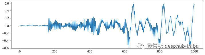
音频数据的格式

# Import librosaimport librosa
# Loads mp3 file with a specific sampling rate, here 16kHzy, sr = librosa.load("c4_sample-1.mp3", sr=16_000)
# Plot the signal stored in 'y'from matplotlib import pyplot as pltimport librosa.display
plt.figure(figsize=(12, 3))plt.title("Audio signal as waveform")librosa.display.waveplot(y, sr=sr);

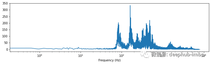
import scipyimport numpy as np
# Applies fast fourier transformation to the signal and takes absolute valuesy_freq = np.abs(scipy.fftpack.fft(y))
# Establishes all possible frequency# (dependent on the sampling rate and the length of the signal)f = np.linspace(0, sr, len(y_freq))
# Plot audio signal as frequency information.plt.figure(figsize=(12, 3))plt.semilogx(f[: len(f) // 2], y_freq[: len(f) // 2])plt.xlabel("Frequency (Hz)")plt.show();

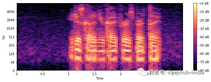
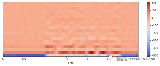
import librosa.display
# Compute short-time Fourier Transformx_stft = np.abs(librosa.stft(y))
# Apply logarithmic dB-scale to spectrogram and set maximum to 0 dBx_stft = librosa.amplitude_to_db(x_stft, ref=np.max)
# Plot STFT spectrogramplt.figure(figsize=(12, 4))librosa.display.specshow(x_stft, sr=sr, x_axis="time", y_axis="log")plt.colorbar(format="%+2.0f dB")plt.show();

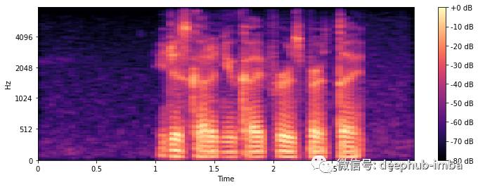
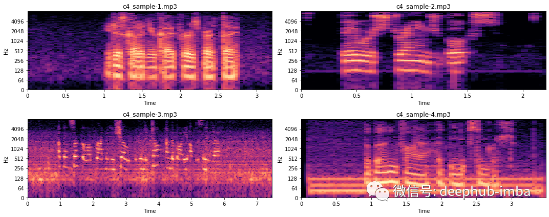
# Compute the mel spectrogramx_mel = librosa.feature.melspectrogram(y=y, sr=sr)
# Apply logarithmic dB-scale to spectrogram and set maximum to 0 dBx_mel = librosa.power_to_db(x_mel, ref=np.max)
# Plot mel spectrogramplt.figure(figsize=(12, 4))librosa.display.specshow(x_mel, sr=sr, x_axis="time", y_axis="mel")plt.colorbar(format="%+2.0f dB")plt.show();

# Extract 'n_mfcc' numbers of MFCCs components (here 20)x_mfccs = librosa.feature.mfcc(y, sr=sr, n_mfcc=20)
# Plot MFCCsplt.figure(figsize=(12, 4))librosa.display.specshow(x_mfccs, sr=sr, x_axis="time")plt.colorbar()plt.show();

数据清洗

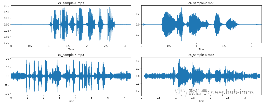
• 大多数录音在录音的开头和结尾都有一段较长的静默期（示例 1 和示例 2）。这是我们在“修剪”时应该注意的事情。
• 在某些情况下，由于按下和释放录制按钮，这些静音期会被“点击”中断（参见示例 2）。
• 一些录音没有这样的静音阶段，即一条直线（示例 3 和 4）。
• 在收听这些录音时，有大量背景噪音。

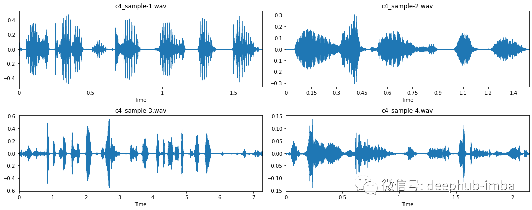
import noisereduce as nrfrom scipy.io import wavfile
# Loop through all four samplesfor i in range(4):
  # Load audio file  fname = "c4_sample-%d.mp3" % (i + 1)  y, sr = librosa.load(fname, sr=16_000)
  # Remove noise from audio sample  reduced_noise = nr.reduce_noise(y=y, sr=sr, stationary=False)
  # Save output in a wav file as mp3 cannot be saved to directly  wavfile.write(fname.replace(".mp3", ".wav"), sr, reduced_noise)

聆听创建的 wav 文件，可以听到噪音几乎完全消失了。虽然我们还引入了更多的代码，但总的来说我们的去噪方法利大于弊。

# Loop through all four samplesfor i in range(4):
  # Load audio file  fname = "c4_sample-%d.wav" % (i + 1)  y, sr = librosa.load(fname, sr=16_000)
  # Trim signal  y_trim, _ = librosa.effects.trim(y, top_db=20)
  # Overwrite previous wav file  wavfile.write(fname.replace(".mp3", ".wav"), sr, y_trim)

特征提取

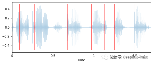
# Extract onset timestamps of wordsonsets = librosa.onset.onset_detect(  y=y, sr=sr, units="time", hop_length=128, backtrack=False)
# Plot onsets together with waveform plotplt.figure(figsize=(8, 3))librosa.display.waveplot(y, sr=sr, alpha=0.2, x_axis="time")for o in onsets:  plt.vlines(o, -0.5, 0.5, colors="r")plt.show()
# Return number of onsetsnumber_of_words = len(onsets)print(f"{number_of_words} onsets were detected in this audio signal.")>>> 7 onsets were detected in this audio signal

duration = len(y) / srwords_per_second = number_of_words / durationprint(f"""The audio signal is {duration:.2f} seconds long,with an average of {words_per_second:.2f} words per seconds.""")
>>> The audio signal is 1.70 seconds long,>>> with an average of 4.13 words per seconds.

# Computes the tempo of a audio recordingtempo = librosa.beat.tempo(y, sr, start_bpm=10)[0]print(f"The audio signal has a speed of {tempo:.2f} bpm.")
>>> The audio signal has a speed of 42.61 bpm.

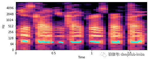
# Extract fundamental frequency using a probabilistic approachf0, _, _ = librosa.pyin(y, sr=sr, fmin=10, fmax=8000, frame_length=1024)
# Establish timepoint of f0 signaltimepoints = np.linspace(0, duration, num=len(f0), endpoint=False)
# Plot fundamental frequency in spectrogram plotplt.figure(figsize=(8, 3))x_stft = np.abs(librosa.stft(y))x_stft = librosa.amplitude_to_db(x_stft, ref=np.max)librosa.display.specshow(x_stft, sr=sr, x_axis="time", y_axis="log")plt.plot(timepoints, f0, color="cyan", linewidth=4)plt.show();

# Computes mean, median, 5%- and 95%-percentile value of fundamental frequencyf0_values = [    np.nanmean(f0),    np.nanmedian(f0),    np.nanstd(f0),    np.nanpercentile(f0, 5),    np.nanpercentile(f0, 95),]print("""This audio signal has a mean of {:.2f}, a median of {:.2f}, astd of {:.2f}, a 5-percentile at {:.2f} and a 95-percentile at {:.2f}.""".format(*f0_values))

>>> This audio signal has a mean of 81.98, a median of 80.46, a>>> std of 4.42, a 5-percentile at 76.57 and a 95-percentile at 90.64.

除以上说的技术以外，还有更多可以探索的音频特征提取技术，这里就不详细说明了。

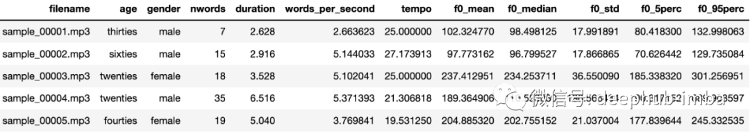
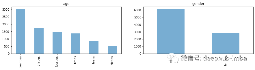
音频数据集的探索性数据分析 (EDA)

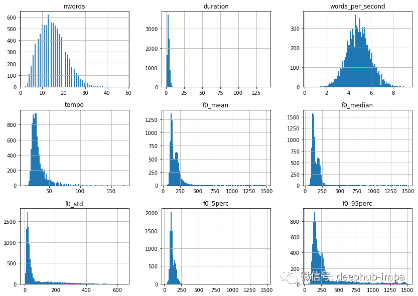
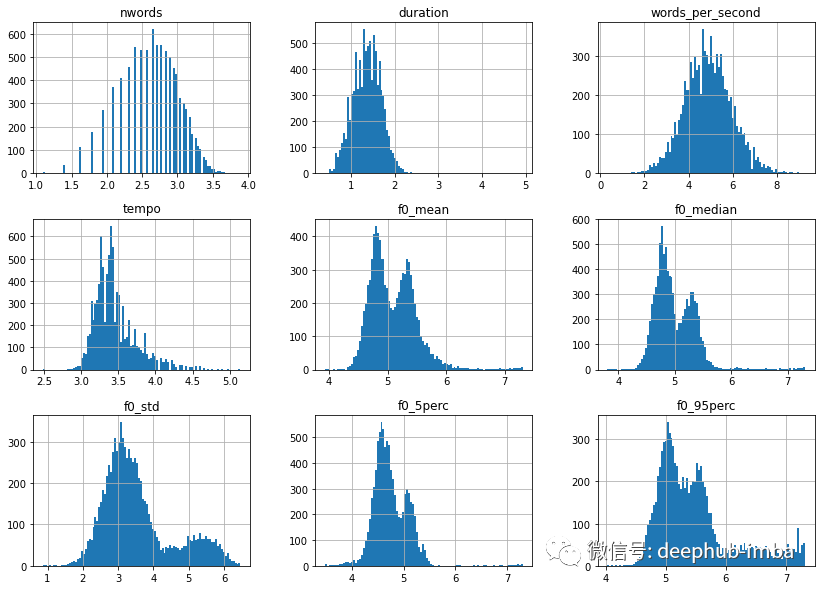
import numpy as np
# Applies log1p on features that are not age, gender, filename or words_per_seconddf = df.apply(    lambda x: np.log1p(x)    if x.name not in ["age", "gender", "filename", "words_per_second"]    else x)
# Let's look at the distribution once moredf.drop(columns=["age", "gender", "filename"]).hist(  bins=100, figsize=(14, 10))plt.show();

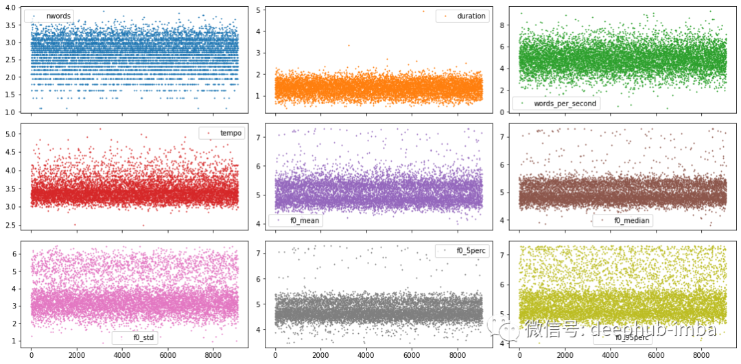
# Plot sample points for each feature individuallydf.plot(lw=0, marker=".", subplots=True, layout=(-1, 3),        figsize=(15, 7.5), markersize=2)plt.tight_layout()plt.show();

# Map age to appropriate numerical valuedf.loc[:, "age"] = df["age"].map({        "teens": 0,        "twenties": 1,        "thirties": 2,        "fourties": 3,        "fifties": 4,        "sixties": 5})
# Map gender to corresponding numerical valuedf.loc[:, "gender"] = df["gender"].map({"male": 0, "female": 1})

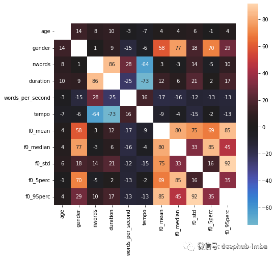
import seaborn as sns
plt.figure(figsize=(8, 8))df_corr = df.corr() * 100sns.heatmap(df_corr, square=True, annot=True, fmt=".0f",            mask=np.eye(len(df_corr)), center=0)plt.show();

模型选择

• 训练我们经典（即浅层）机器学习模型，例如 LogisticRegression 或 SVC。
• 训练深度学习模型，即深度神经网络。
• 使用 TensorflowHub 的预训练神经网络进行特征提取，然后在这些高级特征上训练浅层或深层模型

• CSV 文件中的数据，将其与频谱图中的“mel 强度”特征相结合，并将数据视为表格数据集
• 单独的梅尔谱图并将它们视为图像数据集
• 使用TensorflowHub现有模型提取的高级特征，将它们与其他表格数据结合起来，并将其视为表格数据集

经典（即浅层）机器学习模型

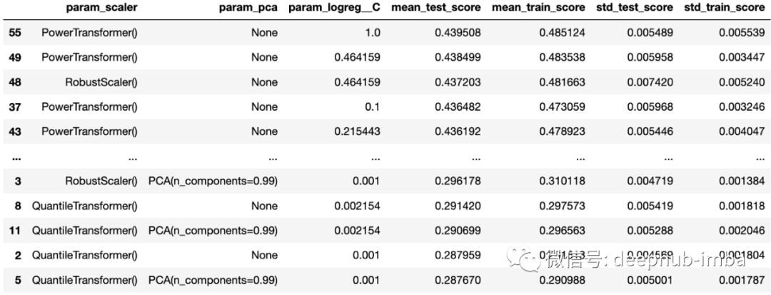
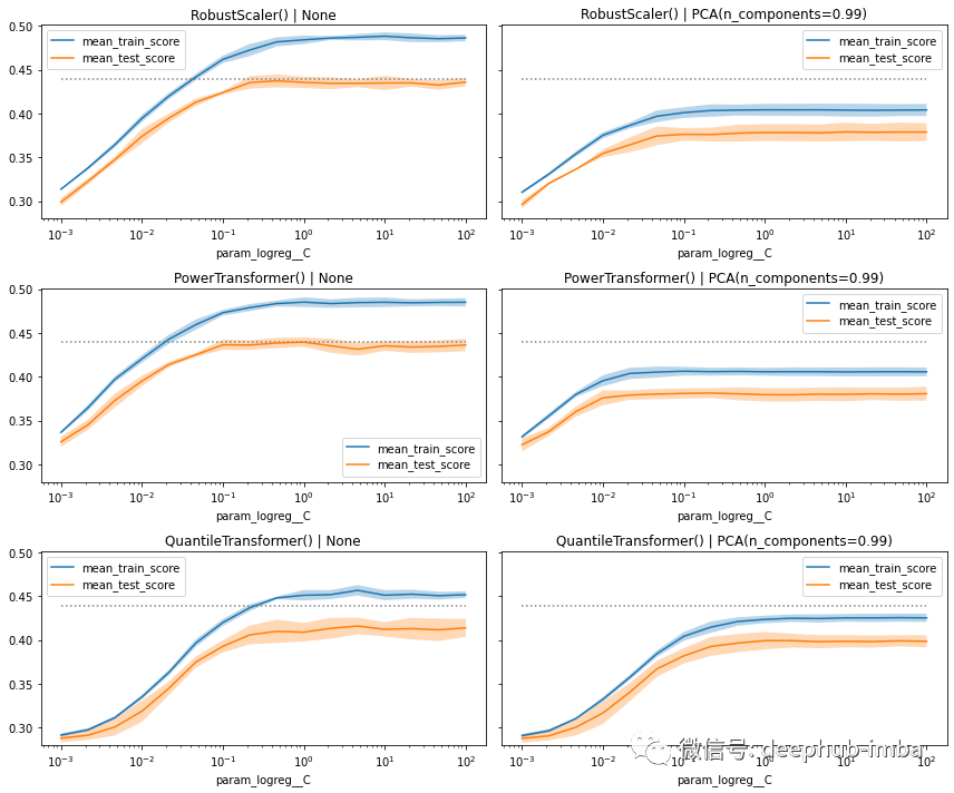
from sklearn.linear_model import LogisticRegressionfrom sklearn.preprocessing import RobustScaler, PowerTransformer, QuantileTransformerfrom sklearn.decomposition import PCAfrom sklearn.pipeline import Pipelinefrom sklearn.model_selection import GridSearchCV
# Create pipelinepipe = Pipeline(    [        ("scaler", RobustScaler()),        ("pca", PCA()),        ("logreg", LogisticRegression(class_weight="balanced")),    ])
# Create gridgrid = {    "scaler": [RobustScaler(), PowerTransformer(), QuantileTransformer()],    "pca": [None, PCA(0.99)],    "logreg__C": np.logspace(-3, 2, num=16),}
# Create GridSearchCVgrid_cv = GridSearchCV(pipe, grid, cv=4, return_train_score=True, verbose=1)
# Train GridSearchCVmodel = grid_cv.fit(x_tr, y_tr)
# Collect results in a DataFramecv_results = pd.DataFrame(grid_cv.cv_results_)
# Select the columns we are interested incol_of_interest = [    "param_scaler",    "param_pca",    "param_logreg__C",    "mean_test_score",    "mean_train_score",    "std_test_score",    "std_train_score",]cv_results = cv_results[col_of_interest]
# Show the dataframe sorted according to our performance metriccv_results.sort_values("mean_test_score", ascending=False)

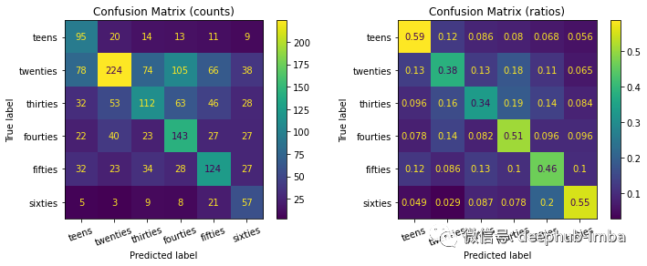
# Compute score of the best model on the withheld test setbest_clf = model.best_estimator_best_clf.score(x_te, y_te)
>>> 0.4354094579008074

总结