基于LSTM-CNN的人体活动识别

来源：DeepHub IMBA
本文约3400字，建议阅读10+分钟
本文带你使用移动传感器产生的原始数据来识别人类活动。

• 下楼
• 上楼
• 跑步
• 坐着
• 站立
• 步行

概述

导入库

from pandas import read_csv, unique
import numpy as np
from scipy.interpolate import interp1dfrom scipy.stats import mode
from sklearn.preprocessing import LabelEncoderfrom sklearn.metrics import classification_report, confusion_matrix, ConfusionMatrixDisplay
from tensorflow import stackfrom tensorflow.keras.utils import to_categoricalfrom keras.models import Sequentialfrom keras.layers import Dense, GlobalAveragePooling1D, BatchNormalization, MaxPool1D, Reshape, Activationfrom keras.layers import Conv1D, LSTMfrom keras.callbacks import ModelCheckpoint, EarlyStoppingimport matplotlib.pyplot as plt%matplotlib inline
import warningswarnings.filterwarnings("ignore")

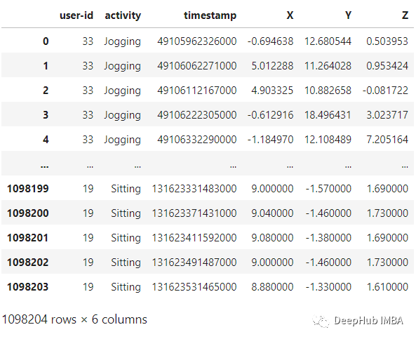
数据集加载和可视化

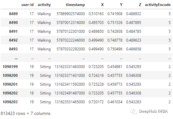
def read_data(filepath):  df = read_csv(filepath, header=None, names=['user-id',                                              'activity',                                              'timestamp',                                              'X',                                              'Y',                                              'Z'])  ## removing ';' from last column and converting it to float  df['Z'].replace(regex=True, inplace=True, to_replace=r';', value=r'')  df['Z'] = df['Z'].apply(convert_to_float)  return df
def convert_to_float(x):  try:      return np.float64(x)  except:      return np.nan
df = read_data('Dataset/WISDM_ar_v1.1/WISDM_ar_v1.1_raw.txt')df

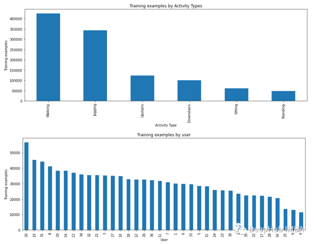
plt.figure(figsize=(15, 5))
plt.xlabel('Activity Type')plt.ylabel('Training examples')df['activity'].value_counts().plot(kind='bar',                                title='Training examples by Activity Types')plt.show()
plt.figure(figsize=(15, 5))plt.xlabel('User')plt.ylabel('Training examples')df['user-id'].value_counts().plot(kind='bar',                                title='Training examples by user')plt.show()

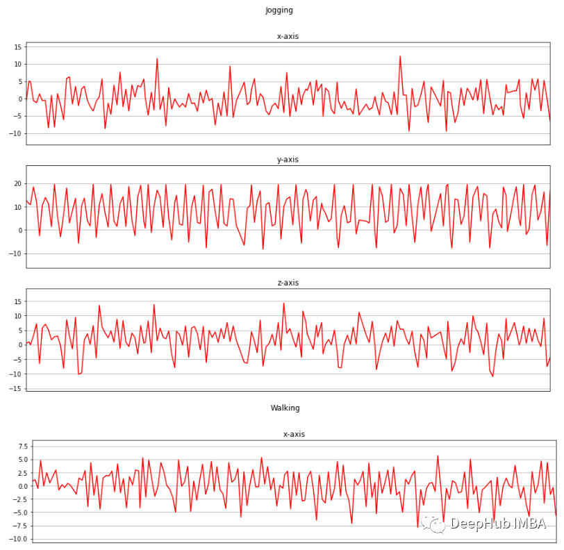
def axis_plot(ax, x, y, title):  ax.plot(x, y, 'r')  ax.set_title(title)  ax.xaxis.set_visible(False)  ax.set_ylim([min(y) - np.std(y), max(y) + np.std(y)])  ax.set_xlim([min(x), max(x)])  ax.grid(True)
for activity in df['activity'].unique():  limit = df[df['activity'] == activity][:180]  fig, (ax0, ax1, ax2) = plt.subplots(nrows=3, sharex=True, figsize=(15, 10))  axis_plot(ax0, limit['timestamp'], limit['X'], 'x-axis')  axis_plot(ax1, limit['timestamp'], limit['Y'], 'y-axis')  axis_plot(ax2, limit['timestamp'], limit['Z'], 'z-axis')  plt.subplots_adjust(hspace=0.2)  fig.suptitle(activity)  plt.subplots_adjust(top=0.9)  plt.show()

数据预处理

• 标签编码
• 线性插值
• 数据分割
• 归一化
• 时间序列分割
• 独热编码

• Downstairs [0]
• Jogging [1]
• Sitting [2]
• Standing [3]
• Upstairs [4]
• Walking [5]

label_encode = LabelEncoder()df['activityEncode'] = label_encode.fit_transform(df['activity'].values.ravel())df

interpolation_fn = interp1d(df['activityEncode'] ,df['Z'], kind='linear')null_list = df[df['Z'].isnull()].index.tolist()for i in null_list:  y = df['activityEncode'][i]  value = interpolation_fn(y)  df['Z']=df['Z'].fillna(value)  print(value)

df_test = df[df['user-id'] > 27]df_train = df[df['user-id'] <= 27]

df_train['X'] = (df_train['X']-df_train['X'].min())/(df_train['X'].max()-df_train['X'].min())df_train['Y'] = (df_train['Y']-df_train['Y'].min())/(df_train['Y'].max()-df_train['Y'].min())df_train['Z'] = (df_train['Z']-df_train['Z'].min())/(df_train['Z'].max()-df_train['Z'].min())df_train

def segments(df, time_steps, step, label_name):  N_FEATURES = 3  segments = []  labels = []  for i in range(0, len(df) - time_steps, step):      xs = df['X'].values[i:i+time_steps]      ys = df['Y'].values[i:i+time_steps]      zs = df['Z'].values[i:i+time_steps]
      label = mode(df[label_name][i:i+time_steps])[0][0]      segments.append([xs, ys, zs])      labels.append(label)
  reshaped_segments = np.asarray(segments, dtype=np.float32).reshape(-1, time_steps, N_FEATURES)  labels = np.asarray(labels)
  return reshaped_segments, labels
TIME_PERIOD = 80STEP_DISTANCE = 40LABEL = 'activityEncode'x_train, y_train = segments(df_train, TIME_PERIOD, STEP_DISTANCE, LABEL)

print('x_train shape:', x_train.shape)print('Training samples:', x_train.shape[0])print('y_train shape:', y_train.shape)
x_train shape: (20334, 80, 3)Training samples: 20334y_train shape: (20334,)

time_period, sensors = x_train.shape[1], x_train.shape[2]num_classes = label_encode.classes_.sizeprint(list(label_encode.classes_))
['Downstairs', 'Jogging', 'Sitting', 'Standing', 'Upstairs', 'Walking']

input_shape = time_period * sensorsx_train = x_train.reshape(x_train.shape[0], input_shape)print("Input Shape: ", input_shape)print("Input Data Shape: ", x_train.shape)
Input Shape: 240Input Data Shape: (20334, 240)

x_train = x_train.astype('float32')y_train = y_train.astype('float32')

y_train_hot = to_categorical(y_train, num_classes)print("y_train shape: ", y_train_hot.shape)y_train shape: (20334, 6)

模型

model = Sequential()model.add(LSTM(32, return_sequences=True, input_shape=(input_shape,1), activation='relu'))model.add(LSTM(32,return_sequences=True, activation='relu'))model.add(Reshape((1, 240, 32)))model.add(Conv1D(filters=64,kernel_size=2, activation='relu', strides=2))model.add(Reshape((120, 64)))model.add(MaxPool1D(pool_size=4, padding='same'))model.add(Conv1D(filters=192, kernel_size=2, activation='relu', strides=1))model.add(Reshape((29, 192)))model.add(GlobalAveragePooling1D())model.add(BatchNormalization(epsilon=1e-06))model.add(Dense(6))model.add(Activation('softmax'))
print(model.summary())

训练和结果

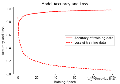
model.compile(loss='categorical_crossentropy', optimizer='adam', metrics=['accuracy'])history = model.fit(x_train,                  y_train_hot,                  batch_size= 192,                  epochs=100                  )

plt.figure(figsize=(6, 4))plt.plot(history.history['accuracy'], 'r', label='Accuracy of training data')plt.plot(history.history['loss'], 'r--', label='Loss of training data')plt.title('Model Accuracy and Loss')plt.ylabel('Accuracy and Loss')plt.xlabel('Training Epoch')plt.ylim(0)plt.legend()plt.show()
y_pred_train = model.predict(x_train)max_y_pred_train = np.argmax(y_pred_train, axis=1)print(classification_report(y_train, max_y_pred_train))

df_test['X'] = (df_test['X']-df_test['X'].min())/(df_test['X'].max()-df_test['X'].min())df_test['Y'] = (df_test['Y']-df_test['Y'].min())/(df_test['Y'].max()-df_test['Y'].min())df_test['Z'] = (df_test['Z']-df_test['Z'].min())/(df_test['Z'].max()-df_test['Z'].min())x_test, y_test = segments(df_test,                        TIME_PERIOD,                        STEP_DISTANCE,                        LABEL)
x_test = x_test.reshape(x_test.shape[0], input_shape)x_test = x_test.astype('float32')y_test = y_test.astype('float32')y_test = to_categorical(y_test, num_classes)

score = model.evaluate(x_test, y_test)print("Accuracy:", score[1])print("Loss:", score[0])

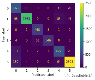
predictions = model.predict(x_test)predictions = np.argmax(predictions, axis=1)y_test_pred = np.argmax(y_test, axis=1)cm = confusion_matrix(y_test_pred, predictions)cm_disp = ConfusionMatrixDisplay(confusion_matrix= cm)cm_disp.plot()plt.show()

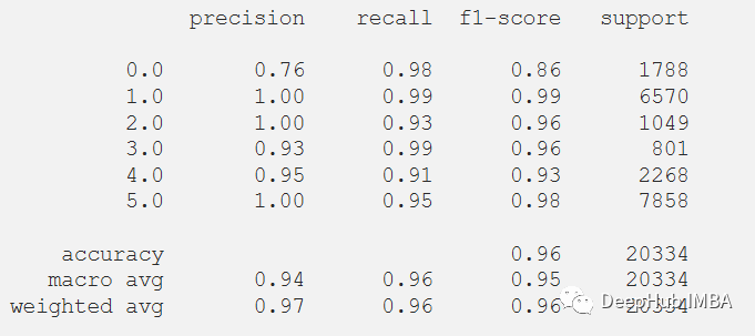
print(classification_report(y_test_pred, predictions))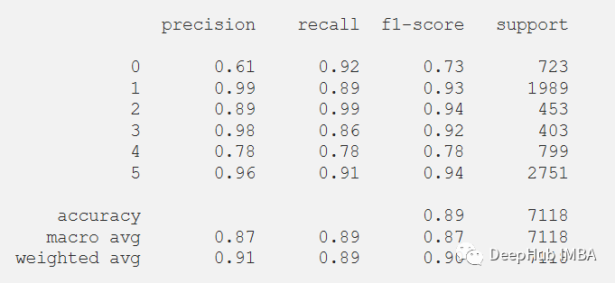

总结