简单好用的深度学习论文绘图专用工具包：Science Plot

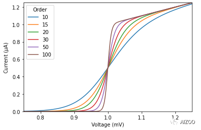
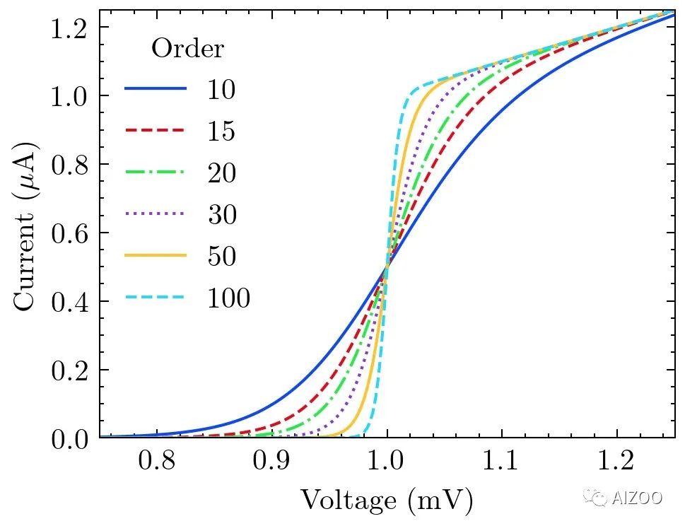
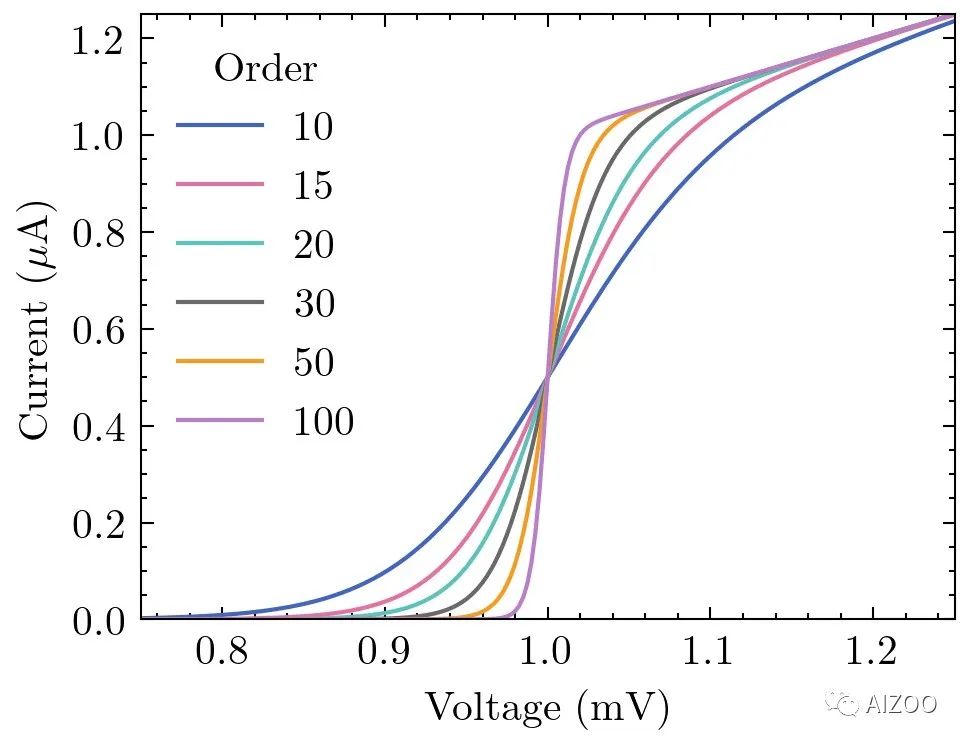
import numpy as npimport matplotlib.pyplot as pltdef model(x, p):    return x ** (2 * p + 1) / (1 + x ** (2 * p))x = np.linspace(0.75, 1.25, 201)

fig, ax = plt.subplots()for p in [10, 15, 20, 30, 50, 100]:          ax.plot(x, model(x, p), label=p)ax.legend(title='Order')ax.set(xlabel='Voltage (mV)')ax.set(ylabel='Current ($\mu$A)')ax.autoscale(tight=True)fig.savefig('fig1.jpg', dpi=300)

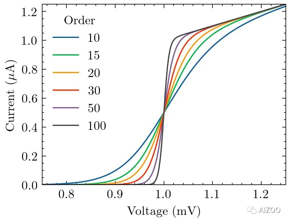
with plt.style.context(['science']):    fig, ax = plt.subplots()        for p in [10, 15, 20, 30, 50, 100]:                       ax.plot(x, model(x, p), label=p)            ax.legend(title='Order')            ax.set(xlabel='Voltage (mV)')            ax.set(ylabel='Current ($\mu$A)')            ax.autoscale(tight=True)            fig.savefig('figures/fig1.pdf')            fig.savefig('figures/fig1.jpg', dpi=300)

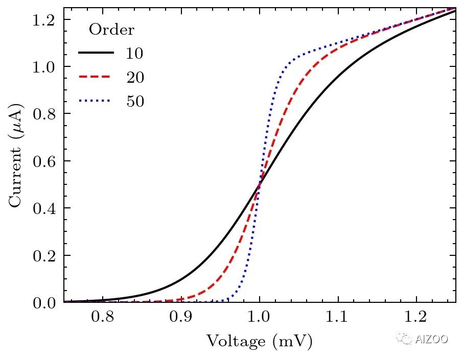
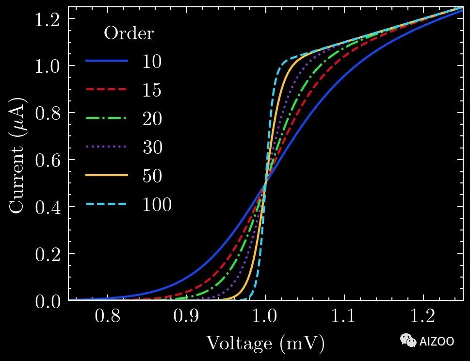
with plt.style.context(['science', 'ieee']):    fig, ax = plt.subplots()    for p in [10, 20, 50]:              ax.plot(x, model(x, p), label=p)           ax.legend(title='Order')        ax.set(xlabel='Voltage (mV)')        ax.set(ylabel='Current ($\mu$A)')        ax.autoscale(tight=True)        fig.savefig('figures/fig2.pdf')        fig.savefig('figures/fig2.jpg', dpi=300)

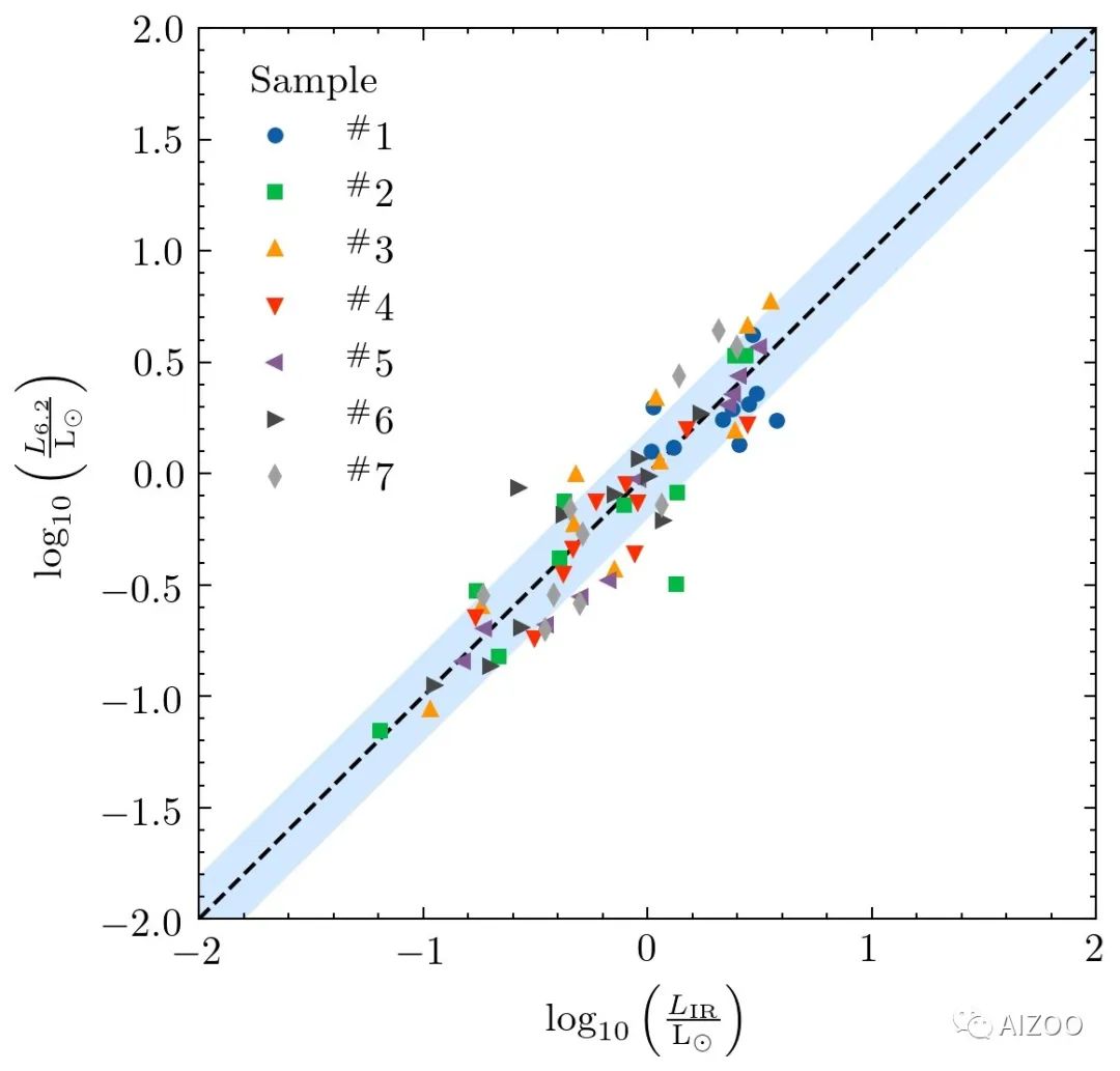
with plt.style.context(['science', 'scatter']):        fig, ax = plt.subplots(figsize=(4,4))        ax.plot([-2, 2], [-2, 2], 'k--')        ax.fill_between([-2, 2], [-2.2, 1.8], [-1.8, 2.2], color='dodgerblue', alpha=0.2, lw=0)    for i in range(7):                x1 = np.random.normal(0, 0.5, 10)                y1 = x1 + np.random.normal(0, 0.2, 10)                ax.plot(x1, y1, label=r"$^\#${}".format(i+1))            ax.legend(title='Sample', loc=2)            ax.set_xlabel(r"$\log_{10}\left(\frac{L_\mathrm{IR}}{\mathrm{L}_\odot}\right)$")            ax.set_ylabel(r"$\log_{10}\left(\frac{L_\mathrm{6.2}}{\mathrm{L}_\odot}\right)$")            ax.set_xlim([-2, 2])            ax.set_ylim([-2, 2])            fig.savefig('figures/fig3.pdf')            fig.savefig('figures/fig3.jpg', dpi=300)