前言

❝
Hello！小伙伴！
非常感谢您阅读海轰的文章，倘若文中有错误的地方，欢迎您指出～
自我介绍 「ଘ(੭ˊᵕˋ)੭」
昵称：海轰
标签：程序猿｜C++选手｜学生
简介：因C语言结识编程，随后转入计算机专业，有幸拿过一些国奖、省奖...已保研。目前正在学习C++/Linux/Python
学习经验：扎实基础 + 多做笔记 + 多敲代码 + 多思考 + 学好英语！初学Python 小白阶段
文章仅作为自己的学习笔记用于知识体系建立以及复习
题不在多学一题懂一题
知其然知其所以然！
❞

1 多元回归

❝
注：这里实在没有找到数据集
引用于：https://blog.csdn.net/HHTNAN/article/details/78843722?utm_source=blogxgwz7
以下代码未验证
❞

1.1 选取数据

import pandas as pd
import seaborn as sns
import matplotlib.pyplot as plt
import matplotlib as mpl   #显示中文
def mul_lr():
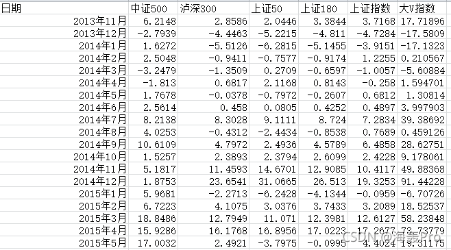
    pd_data=pd.read_excel('../profile/test.xlsx')
    print('pd_data.head(10)=\n{}'.format(pd_data.head(10)))
font = {
    "family": "Microsoft YaHei"
}
matplotlib.rc("font", **font)
mpl.rcParams['axes.unicode_minus']=False 
sns.pairplot(pd_data, x_vars=['中证500','泸深300','上证50','上证180'], y_vars='上证指数',kind="reg", size=5, aspect=0.7)
plt.show()

1.2 构建训练集与测试集，并构建模型

from sklearn.model_selection import train_test_split #这里是引用了交叉验证
from sklearn.linear_model import LinearRegression  #线性回归
from sklearn import metrics
import numpy as np
import matplotlib.pyplot as plt
def mul_lr():   #续前面代码
    #剔除日期数据，一般没有这列可不执行，选取以下数据http://blog.csdn.net/chixujohnny/article/details/51095817
    X=pd_data.loc[:,('中证500','泸深300','上证50','上证180')]
    y=pd_data.loc[:,'上证指数']
    X_train,X_test, y_train, y_test = train_test_split(X,y,test_size = 0.2,random_state=100)
    print ('X_train.shape={}\n y_train.shape ={}\n X_test.shape={}\n,  y_test.shape={}'.format(X_train.shape,y_train.shape, X_test.shape,y_test.shape))
    linreg = LinearRegression()
    model=linreg.fit(X_train, y_train)
    print (model)
    # 训练后模型截距
    print (linreg.intercept_)
    # 训练后模型权重（特征个数无变化）
    print (linreg.coef_)

1.3 模型预测

#预测
y_pred = linreg.predict(X_test)
print (y_pred) #10个变量的预测结果

1.4 模型评估

    #评价
    #(1) 评价测度
    # 对于分类问题，评价测度是准确率，但这种方法不适用于回归问题。我们使用针对连续数值的评价测度(evaluation metrics)。
    # 这里介绍3种常用的针对线性回归的测度。
    # 1)平均绝对误差(Mean Absolute Error, MAE)
    # (2)均方误差(Mean Squared Error, MSE)
    # (3)均方根误差(Root Mean Squared Error, RMSE)
    # 这里我使用RMES。
    sum_mean=0
    for i in range(len(y_pred)):
        sum_mean+=(y_pred[i]-y_test.values[i])**2
    sum_erro=np.sqrt(sum_mean/10)  #这个10是你测试级的数量
    # calculate RMSE by hand
    print ("RMSE by hand:",sum_erro)
    #做ROC曲线
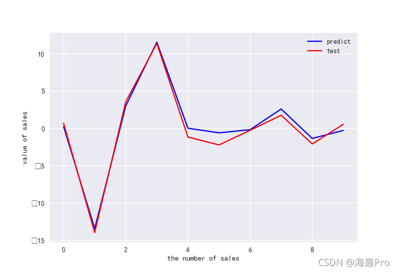
    plt.figure()
      plt.plot(range(len(y_pred)),y_pred,'b',label="predict")
     plt.plot(range(len(y_pred)),y_test,'r',label="test")
    plt.legend(loc="upper right") #显示图中的标签
    plt.xlabel("the number of sales")
    plt.ylabel('value of sales')
    plt.show()

2 logistic回归

2.1 鸢尾花数据集

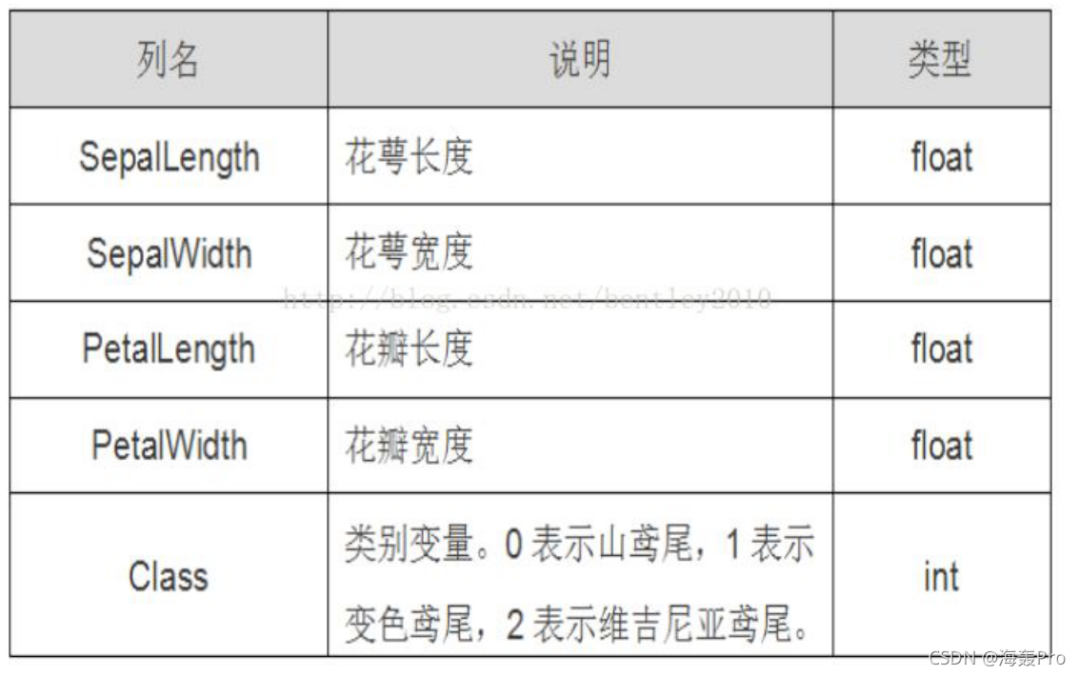
鸢尾花有三个亚属，分别是山鸢尾（Iris-setosa）、变色鸢尾（Iris- versicolor）和维吉尼亚鸢尾（Iris-virginica）。

该数据集一共包含4个特征变量，1个类别变量。共有150个样本，iris是鸢尾植物，这里存储了其萼片和花瓣的长宽，共4个属性，鸢尾植物分三类。

2.2 绘制散点图

Demo代码

import matplotlib.pyplot as plt 
import numpy as np 
from sklearn.datasets import load_iris 
iris = load_iris()
#获取花卉两列数据集  
DD = iris.data  
X = [x[0] for x in DD]  
Y = [x[1] for x in DD] 
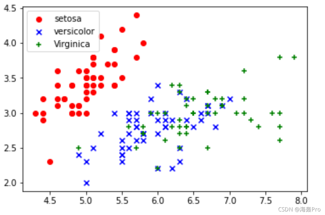
plt.scatter(X[:50], Y[:50], color='red', marker='o', label='setosa') 
plt.scatter(X[50:100], Y[50:100], color='blue', marker='x', label='versicolor') 
plt.scatter(X[100:], Y[100:],color='green', marker='+', label='Virginica') 
plt.legend(loc=2) #左上角 
plt.show()

运行结果

2.3 逻辑回归分析

Demo代码

from sklearn.linear_model import LogisticRegression 
iris = load_iris() 
X = iris.data[:, :2]   #获取花卉两列数据集 
Y = iris.target 
lr = LogisticRegression(C=1e5)    
lr.fit(X,Y) 
#meshgrid函数生成两个网格矩阵  
h = .02  
x_min, x_max = X[:, 0].min()-.5, X[:, 0].max()+.5 
y_min, y_max = X[:, 1].min()-.5, X[:, 1].max()+.5 
xx, yy = np.meshgrid(np.arange(x_min, x_max, h), np.arange(y_min, y_max, h)) 
Z = lr.predict(np.c_[xx.ravel(), yy.ravel()]) 
Z = Z.reshape(xx.shape)  
plt.figure(1, figsize=(8,6))  
plt.pcolormesh(xx, yy, Z, cmap=plt.cm.Paired) 
plt.scatter(X[:50,0], X[:50,1], color='red',marker='o', label='setosa')  
plt.scatter(X[50:100,0], X[50:100,1], color='blue', marker='x', label='versicolor')
plt.scatter(X[100:,0], X[100:,1], color='green', marker='s', label='Virginica') 
plt.xlabel('Sepal length')  
plt.ylabel('Sepal width')  
plt.xlim(xx.min(), xx.max())  
plt.ylim(yy.min(), yy.max())  
plt.xticks(())  
plt.yticks(())  
plt.legend(loc=2)   
plt.show()

运行结果

结语

学习来源：B站及其课堂PPT，对其中代码进行了复现

❝
https://www.bilibili.com/video/BV12h411d7Dm
参考资料：https://blog.csdn.net/HHTNAN/article/details/78843722?utm_source=blogxgwz7
❞

「文章仅作为学习笔记，记录从0到1的一个过程」

希望对您有所帮助，如有错误欢迎小伙伴指正～

Python数学建模系列（九）：回归

前言