
SCI绘图-网络图可视化最详细教程!
大家好,我是半岛小铁盒!在上期内容💥 SCI绘图-网络(Graph)图可视化工具合集 👈中,介绍了网络图的原理和基本组成以及常用的网络图的可视化工具推荐,那么本期内容将为大家带来网络图可视化分析实战,通过讲解igraph的基本使用让大家进一步理解网络图(Graph)的概念,最后使用ggraph来绘制好看的网络图。
Tips:后续文中提及的 Nodes 或 Verticles 都表示节点,顶点与节点同义。
安装依赖包
使用R包安装命令`install.packages`分别安装 igraph 和 ggraph依赖包
        install.packages("igraph")


        install.packages("ggraph")
igraph 包的基本使用
⭐通过 igraph 来理解 Graph 图中的节点(Nodes)、边(Edges)、布局(Layouts)、度(Degree)以及 节点和边的重要性等。
导包创建 Graph 1.常见方式
library(igraph)
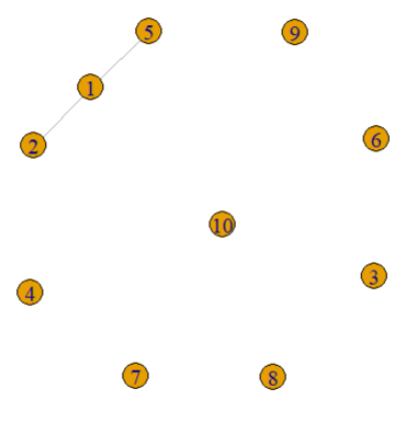
eg. 构建一个包含10个节点(编号为 1 到 10)和连接节点1-2 和1-5的两条边的网络
        g <- make_graph(edges = c(1,2, 1,5), n=10, directed = FALSE)


        plot(g)
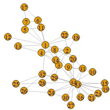
使用内置的网络数据,创建 Graph
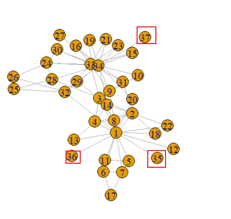
        g <- make_graph('Zachary')


        plot(g)
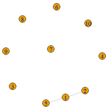
公式以 ~ 开头, edge操作符使用 + 或 - 表示,其中 - 为无向边,+ 表示箭头,‘-+’ 等价于 ‘->’ 。
        g <- make_graph(~ 1-2, 1-5, 3, 4, 5, 6, 7, 8, 9, 10)


        plot(g)
节点和边在igraph中具有数字ID,对于具有n个节点的图,节点ID始终介于1和n之间,边ID始终介于1和m(图中边的总数)之间。
g <- make_graph('Zachary')
添加节点和边
        # 添加3个新的节点


        g <- add_vertices(g, 3)


        g <- add_edges(g, edges = c(1,35, 1,36, 34,37))


        plot(g)
在igraph中可以使用magrittr包中的运算符 %>%
        # 添加节点和边


        g <- g %>%


          add_edges(edges=c(1,34)) %>%


          add_vertices(3) %>%


          add_edges(edges=c(38,39, 39,40, 40,38, 40,37))
删除节点和边,使用delete_vertices 和delete_edges 来执行删除操作
节点和边的其他属性
        # 例如删除连接顶点1-34的边,获取其ID然后删除


        ids <- get.edge.ids(g, c(1,34))


        g <- delete_edges(g, ids)
除了ID之外,顶点和边还具有具有名称、绘图坐标、元数据和权重等属性
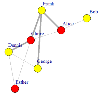
        # 使用公式法创建图


        g <- make_graph(~ Alice-Bob:Claire:Frank,


                          Claire-Alice:Dennis:Frank:Esther,


                          George-Dennis:Frank, Dennis-Esther)


        plot(g)
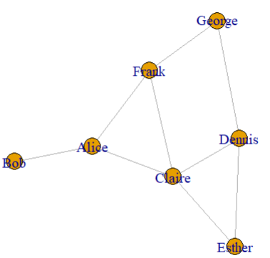
V 和 E 分别是获取所有顶点和边的标准方法
        > V(g)


        + 7/7 vertices, named, from 8419d0d:


        [1] Alice  Bob    Claire Frank  Dennis Esther George


        > E(g)


        + 9/9 edges from 8419d0d (vertex names):


        [1] Alice --Bob    Alice --Claire Alice --Frank  Claire--Frank  Claire--Dennis


        [6] Claire--Esther Frank --George Dennis--Esther Dennis--Georg
设置节点和边的属性值
度 Degree
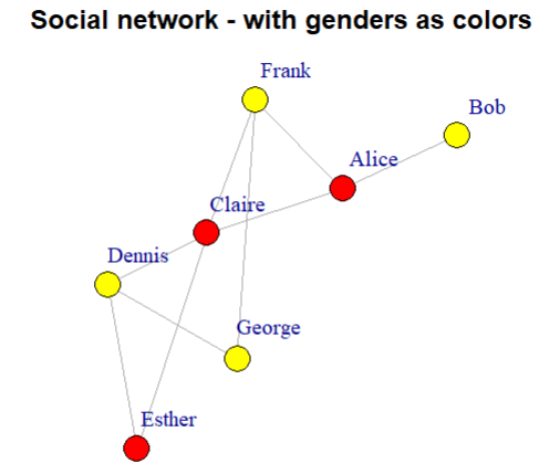
        V(g)$age <- c(25, 31, 18, 23, 47, 22, 50)


        V(g)$gender <- c("f", "m", "f", "m", "m", "f", "m")


        E(g)$is_formal <- c(FALSE, FALSE, TRUE, TRUE, TRUE, FALSE, TRUE, FALSE, FALSE)


        > summary(g)


        IGRAPH 8419d0d UN-- 7 9 --


        + attr: name (v/c), age (v/n), gender (v/c), is_formal (e/l)


        # 删除节点的age属性


        g <- delete_vertex_attr(g, "gender"
度指的是节点所连接的边的数量
介数中心性 找出对网络重要的边
        > degree(g)


         Alice    Bob Claire  Frank Dennis Esther George


             3      1      4      3      3      2      2


        # get by ID or name


        degree(g, v=c(3,4,5))


        degree(g, v=c("Carmina", "Frank", "Dennis"))
布局
        > ebs <- edge_betweenness(g)


        > as_edgelist(g)[ebs == max(ebs), ]


             [,1]    [,2]


        [1,] "Alice" "Bob"


        [2,] "Alice" "Claire"
以下是igraph中的所有布局算法,建议提前了解下,在ggraph中也支持igraph中的布局。
| 布局名称 | 算法描述 |
|---|---|
layout_randomly | Places the vertices completely randomly |
layout_in_circle | Deterministic layout that places the vertices on a circle |
layout_on_sphere | Deterministic layout that places the vertices evenly on the surface of a sphere |
layout_with_drl | The Drl (Distributed Recursive Layout) algorithm for large graphs |
layout_with_fr | Fruchterman-Reingold force-directed algorithm |
layout_with_kk | Kamada-Kawai force-directed algorithm |
layout_with_lgl | The LGL (Large Graph Layout) algorithm for large graphs |
layout_as_tree | Reingold-Tilford tree layout, useful for (almost) tree-like graphs |
layout_nicely | Layout algorithm that automatically picks one of the other algorithms based on certain properties of the graph |
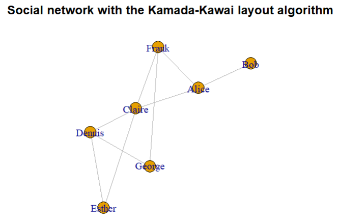
        layout <- layout_with_kk(g)


        plot(g, layout = layout,


             main = "Social network with the Kamada-Kawai layout algorithm")
绘图时节点、边的颜色、大小有很多参数可以调控,这里就不一一介绍了,具体可参见包的帮助文档。
          # set style of nodes


        V(g)$color <- ifelse(V(g)$gender == "m", "yellow", "red")


        plot(g, layout = layout, vertex.label.dist = 3.5,


             main = "Social network - with genders as colors")
          # set edge width


        plot(g, layout=layout, vertex.label.dist=3.5, vertex.size=20,


        vertex.color=ifelse(V(g)$gender == "m", "yellow", "red"),


        edge.width=ifelse(E(g)$is_formal, 5, 1))
使用 ggraph 包 绘制网络图
ggraph 是 ggplot2 的扩展,旨在支持关系数据结构,例如网络、图和树。可以使用ggplot2来绘图,十分轻量和简便。
ggraph 需要结合 tidygraph来使用,tidygraph中 的 tbl_graph 类是 igraph 对象的封装,用来加载网络图的数据,不仅提供使用 tidy API 操作的方法,而且作为igraph 的子类可以调用父类的方法。
载包
        library(ggraph)


        library(tidygraph)
使用 tidygraph 的 as_tbl_graph 方法加载绘图数据
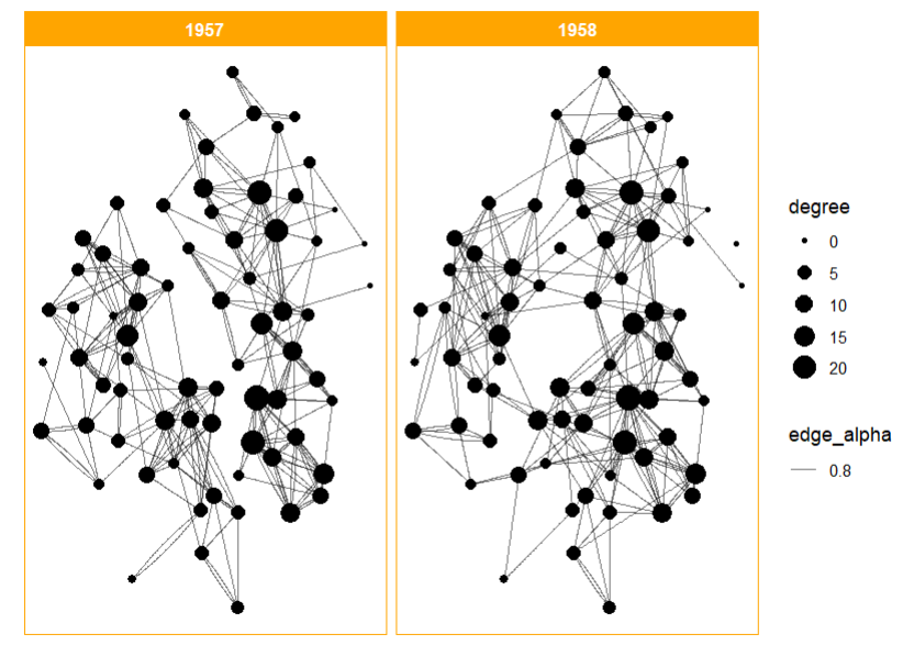
          # 内置数据集 highschool


        > class(highschool)


        [1] "data.frame"


        > head(highschool)


          from to year


        1    1 14 1957


        2    1 15 1957


        3    1 21 1957


        4    1 54 1957


        5    1 55 1957


        6    2 21 1957


        # 生成 tbl_graph对象用于后续绘图


        > gr <- as_tbl_graph(highschool)


        > gr


        # A tbl_graph: 70 nodes and 506 edges


        #


        # A directed multigraph with 1 component
tbl_graph 可以被视为两个链接表(Nodes 和 Edges)的集合,因此有必要指定在操作期间引用哪个表, 使用activate 函数定义当前是否正在操作节点数据或边数据,其中默认激活的是节点数据。
        gr <- gr |>


          # 在Nodes表中添加一列 degree数据


          mutate(degree = centrality_degree(mode = 'in'))
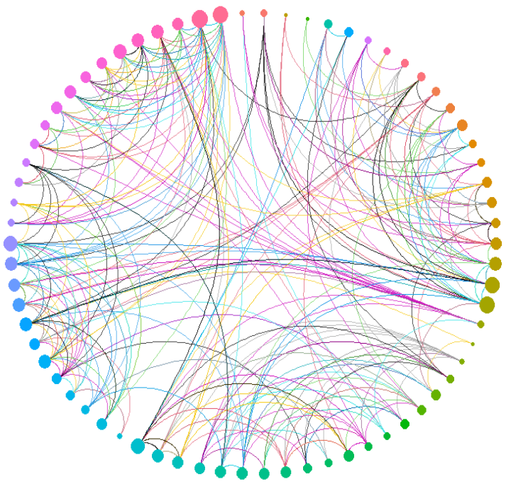
使用ggraph绘制第一张网络图
          # 采用 igraph中相同的 Kamada-Kawai force-directed algorithm布局


        ggr <- ggraph(gr, layout = 'kk') +


            # 绘制透明度0.8且带一点弧度的边


            geom_edge_fan(aes(alpha = 0.8)) +


            # 节点的大小表示degree


            geom_node_point(aes(size = degree)) +


            # 按照年份 切分子图


            facet_edges(~year) +


            # 设置主题


            theme_graph(foreground = 'orange', fg_text_colour = 'white')
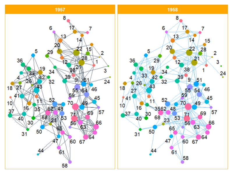
        ggr +


          geom_edge_fan0(aes(colour = year), alpha = 0.8,


          show.legend = FALSE) +


          geom_node_point(aes(size = degree, colour = factor(name)),


          show.legend = FALSE) +


          geom_node_text(aes(label=name), repel = T)+


          facet_edges(~year) +


          theme_graph(foreground = 'orange', fg_text_colour = 'white')
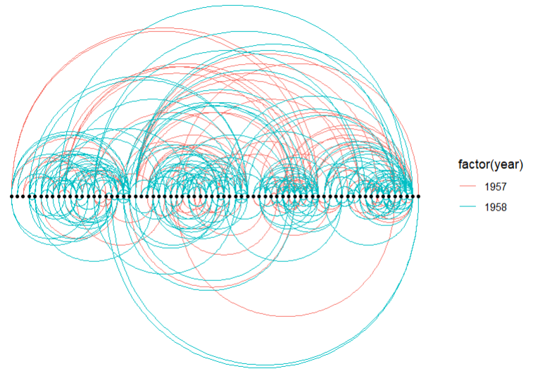
更换布局
          # 设置 margin


        set_graph_style(plot_margin = margin(1,1,1,1))


          # linear layout


        ggraph(graph, layout = 'linear') +


          geom_edge_arc(aes(colour = factor(year))) +


          geom_node_point(size=1) +


          theme_graph(fg_text_colour = 'white')
circular layout
        ggraph(graph, layout = 'linear', circular = TRUE) +


          geom_edge_arc(aes(colour = from), alpha=0.7) +


          scale_edge_colour_identity() +


          geom_node_point(aes(size = degree, colour = factor(name)),


                          show.legend = FALSE) +


          theme_graph(fg_text_colour = 'white')
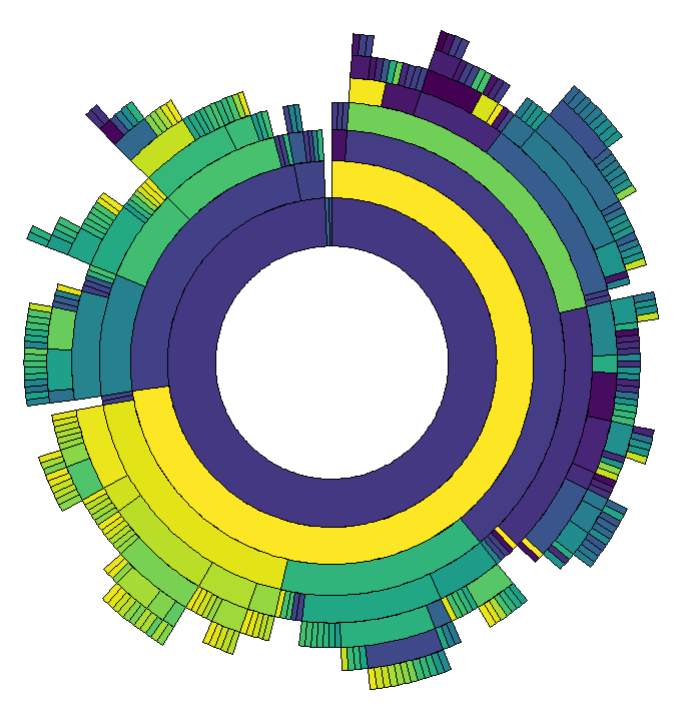
partition circular lay o ut
        ggraph(graph, 'partition', circular = TRUE) +


          geom_node_arc_bar(aes(fill = name), size = 0.25,


                            show.legend = FALSE) +


          scale_fill_viridis_d() +


          coord_fixed()
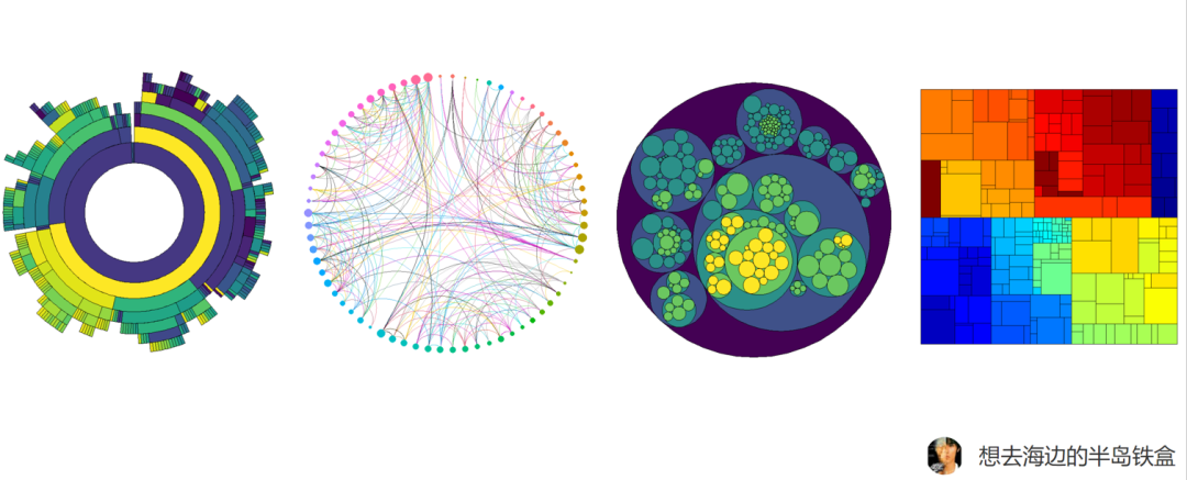
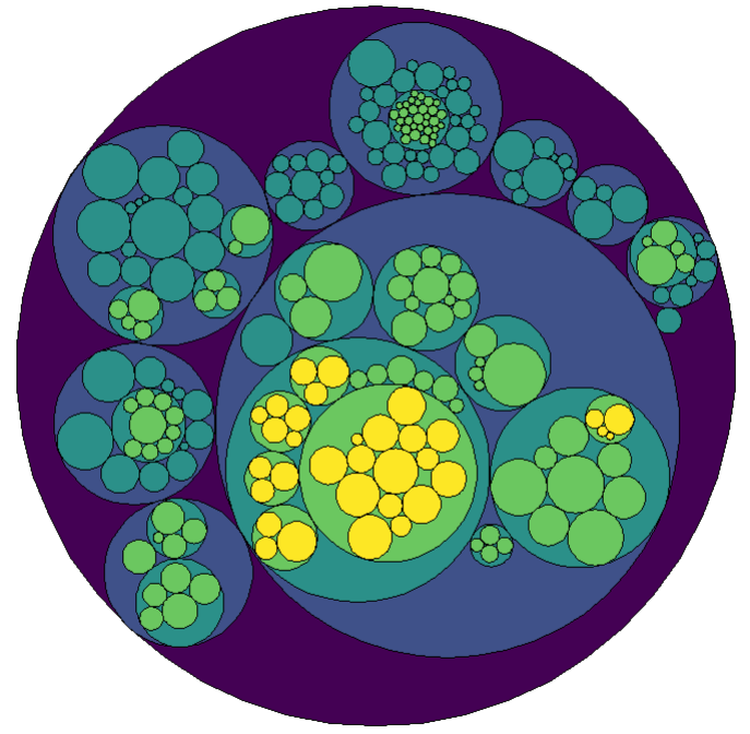
circlepack lay o ut
        graph <- tbl_graph(flare$vertices, flare$edges)


        set.seed(1)


        ggraph(graph, 'circlepack', weight = size) +


          geom_node_circle(aes(fill = depth), size = 0.25, n = 50,


                           show.legend = FALSE) +


          scale_fill_viridis_c() +


          coord_fixed() +


          theme_graph(fg_text_colour = 'white')
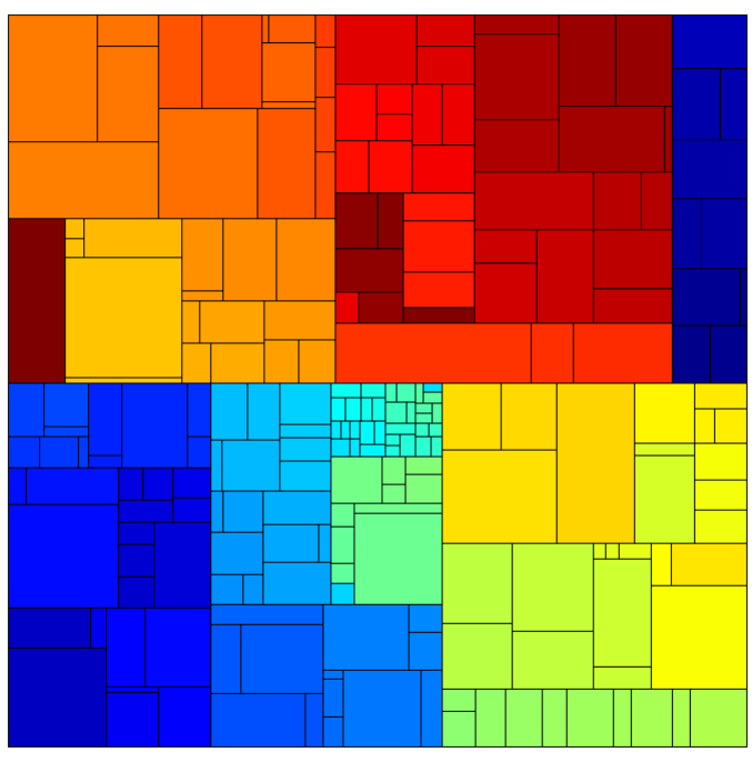
tr eemap lay o ut
        ggraph(graph, 'treemap', weight = size) +


          geom_node_tile(aes(fill = name), size = 0.25,


                         show.legend = FALSE) +


          scale_fill_manual(values = jet.colors(252)) +


          theme_graph(fg_text_colour = 'white')
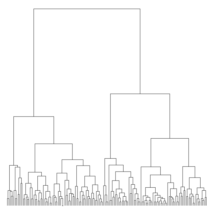
dendrogram lay o ut
        dendrogram <- hclust(dist(iris[, 1:4]))


        ggraph(dendrogram, 'dendrogram', height = height) +


          geom_edge_elbow() +


          theme_graph(fg_text_colour = 'white')
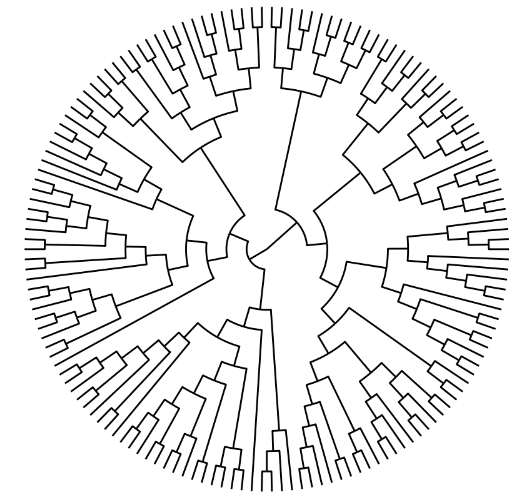
        ggraph(dendrogram, 'dendrogram', circular = TRUE) +


          geom_edge_elbow() +


          coord_fixed()+


          theme_graph(fg_text_colour = 'white')
网络图可视化小结 >>>
网络图的可视化包和绘图方法五花八门,只要掌握其中的逻辑操作起来都是千篇一律!当然,图形的美观这方面的调节还是需要个人天赋,实在不行找篇文献的样图模仿便是了!ggplot2提供了很棒的底层方法,让网络图的绘制轻量简便。只要你肯费些功夫,一定能绘制出好看的SCI图 。

点赞👍关注
本期就介绍到这里啦!持续更新ING~

整理不易,期待您的点赞、分享、转发...

往期精彩推荐
SCI绘图-网络(Graph)图可视化工具合集 龙年微信红包封面!限量2000份! 科研论文还不知道如何配色2? 科研论文还不知道如何配色1? SCI绘图-ggplot绘制超好看的火山图 HTTPX,一个超强的爬虫库! GSEA分析实战及结果可视化教程! 一文读懂GSEA分析原理 SCI绘图-箱线图的绘制原理与方法
更多合集推荐
🔥#SCI绘图 💥 #生物信息 ✨ #科研绘图素材资源 📚 #数学 🌈 #测序原理
我知道你
在看
哦
