
用 Python 动态可视化,看看比特币这几年
来源:早起Python 本文约3600字,建议阅读8分钟
比特币一年翻6倍?


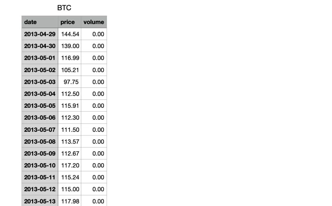
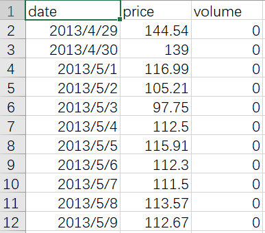
import requestsimport jsonimport csvimport timetime_stamp = int(time.time())url = f"https://web-api.coinmarketcap.com/v1/cryptocurrency/ohlcv/historical?convert=USD&slug=bitcoin&time_end={time_stamp}&time_start=1367107200"rd = requests.get(url = url)# 返回的数据是 JSON 格式,使用 json 模块解析co = json.loads(rd.content)list1 = co['data']['quotes']with open('BTC.csv','w' ,encoding='utf8',newline='') as f:csvi = csv.writer(f)csv_head = ["date","price","volume"]csvi.writerow(csv_head)for i in list1:quote_date = i["time_open"][:10]quote_price = "{:.2f}".format(i["quote"]["USD"]["close"])quote_volume = "{:.2f}".format(i["quote"]["USD"]["volume"])csvi.writerow([quote_date, quote_price, quote_volume])
import pandas as pdimport matplotlib as mplfrom matplotlib import cmimport numpy as npimport matplotlib.pyplot as pltimport matplotlib.ticker as tickerimport matplotlib.animation as animationfrom IPython.display import HTMLfrom datetime import datetimeplt.rcParams['font.sans-serif'] = ['SimHei']plt.rcParams['axes.unicode_minus'] = Falseplt.rc('axes',axisbelow=True)mpl.rcParams['animation.embed_limit'] = 2**128
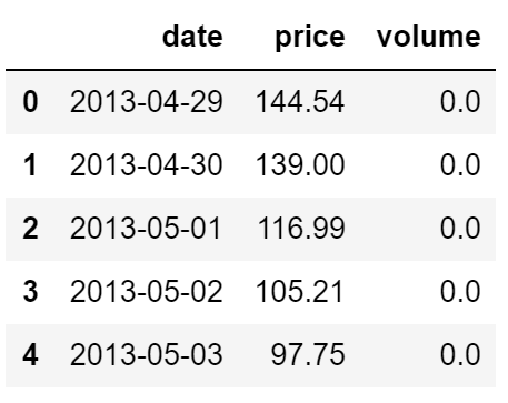
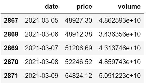
df = pd.read_csv('BTC.csv')df['date']=[datetime.strptime(d, '%Y/%m/%d').date() for d in df['date']]
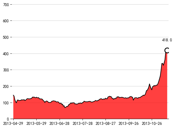
Span=180N_Span=0df_temp=df.loc[N_Span*Span:(N_Span+1)*Span,:]df_temp.head(5)fig =plt.figure(figsize=(6,4), dpi=100)plt.subplots_adjust(top=1,bottom=0,left=0,right=0.9,hspace=0,wspace=0)plt.fill_between(df_temp.date.values, y1=df_temp.price.values, y2=0,alpha=0.75, facecolor='r', linewidth=1,edgecolor ='none',zorder=1)plt.plot(df_temp.date, df_temp.price, color='k',zorder=2)plt.scatter(df_temp.date.values[-1], df_temp.price.values[-1], color='white',s=150,edgecolor ='k',linewidth=2,zorder=3)plt.text(df_temp.date.values[-1], df_temp.price.values[-1]*1.18,s=np.round(df_temp.price.values[-1],1),size=10,ha='center', va='top')plt.ylim(0, df_temp.price.max()*1.68)plt.xticks(ticks=df_temp.date.values[0:Span+1:30],labels=df_temp.date.values[0:Span+1:30],rotation=0)plt.margins(x=0.01)ax = plt.gca()#获取边框ax.spines['top'].set_color('none') # 设置上‘脊梁’为无色ax.spines['right'].set_color('none') # 设置上‘脊梁’为无色ax.spines['left'].set_color('none') # 设置上‘脊梁’为无色plt.grid(axis="y",c=(217/256,217/256,217/256),linewidth=1) #设置网格线plt.show()
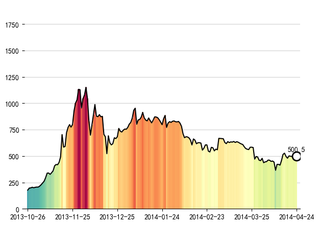
Span_Date =180Num_Date =360 #终止日期df_temp=df.loc[Num_Date-Span_Date: Num_Date,:] #选择从Num_Date-Span_Date开始到Num_Date的180天的数据colors = cm.Spectral_r(df_temp.price / float(max(df_temp.price)))fig =plt.figure(figsize=(6,4), dpi=100)plt.subplots_adjust(top=1,bottom=0,left=0,right=0.9,hspace=0,wspace=0)plt.bar(df_temp.date.values,df_temp.price.values,color=colors,width=1,align="center",zorder=1)plt.plot(df_temp.date, df_temp.price, color='k',zorder=2)plt.scatter(df_temp.date.values[-1], df_temp.price.values[-1], color='white',s=150,edgecolor ='k',linewidth=2,zorder=3)plt.text(df_temp.date.values[-1], df_temp.price.values[-1]*1.18,s=np.round(df_temp.price.values[-1],1),size=10,ha='center', va='top')plt.ylim(0, df_temp.price.max()*1.68)plt.xticks(ticks=df_temp.date.values[0: Span_Date +1:30],labels=df_temp.date.values[0: Span_Date +1:30],rotation=0)plt.margins(x=0.01)ax = plt.gca()#获取边框ax.spines['top'].set_color('none') # 设置上‘脊梁’为无色ax.spines['right'].set_color('none') # 设置上‘脊梁’为无色ax.spines['left'].set_color('none') # 设置上‘脊梁’为无色plt.grid(axis="y",c=(217/256,217/256,217/256),linewidth=1) #设置网格线plt.show()
动态可视化
def draw_areachart(Num_Date):Span_Date=180ax.clear()if Num_Date<Span_Date:df_temp=df.loc[0:Num_Date,:]df_span=df.loc[0:Span_Date,:]colors = cm.Spectral_r(df_span.price.values / float(max(df_span.price.values)))plt.bar(df_temp.date.values,df_temp.price.values,color=colors,width=1.5,align="center",zorder=1)plt.plot(df_temp.date, df_temp.price, color='k',zorder=2)plt.scatter(df_temp.date.values[-1], df_temp.price.values[-1], color='white',s=150,edgecolor ='k',linewidth=2,zorder=3)plt.text(df_temp.date.values[-1], df_temp.price.values[-1]*1.18,s=np.round(df_temp.price.values[-1],1),size=10,ha='center', va='top')plt.ylim(0, df_span.price.max()*1.68)plt.xlim(df_span.date.values[0], df_span.date.values[-1])plt.xticks(ticks=df_span.date.values[0:Span_Date+1:30],labels=df_span.date.values[0:Span_Date+1:30],rotation=0,fontsize=9)else:df_temp=df.loc[Num_Date-Span_Date:Num_Date,:]colors = cm.Spectral_r(df_temp.price / float(max(df_temp.price)))plt.bar(df_temp.date.values[:-2],df_temp.price.values[:-2],color=colors[:-2],width=1.5,align="center",zorder=1)plt.plot(df_temp.date[:-2], df_temp.price[:-2], color='k',zorder=2)plt.scatter(df_temp.date.values[-4], df_temp.price.values[-4], color='white',s=150,edgecolor ='k',linewidth=2,zorder=3)plt.text(df_temp.date.values[-1], df_temp.price.values[-1]*1.18,s=np.round(df_temp.price.values[-1],1),size=10,ha='center', va='top')plt.ylim(0, df_temp.price.max()*1.68)plt.xlim(df_temp.date.values[0], df_temp.date.values[-1])plt.xticks(ticks=df_temp.date.values[0:Span_Date+1:30],labels=df_temp.date.values[0:Span_Date+1:30],rotation=0,fontsize=9)plt.margins(x=0.2)ax.spines['top'].set_color('none') # 设置上‘脊梁’为红色ax.spines['right'].set_color('none') # 设置上‘脊梁’为无色ax.spines['left'].set_color('none') # 设置上‘脊梁’为无色plt.grid(axis="y",c=(217/256,217/256,217/256),linewidth=1) #设置网格线plt.text(0.01, 0.95,"BTC平均价格($)",transform=ax.transAxes, size=10, weight='light', ha='left')ax.text(-0.07, 1.03, '2013年到2021年的比特币BTC价格变化情况',transform=ax.transAxes, size=17, weight='light', ha='left')fig, ax = plt.subplots(figsize=(6,4), dpi=100)plt.subplots_adjust(top=1,bottom=0.1,left=0.1,right=0.9,hspace=0,wspace=0)draw_areachart(150)
import matplotlib.animation as animationfrom IPython.display import HTMLfig, ax = plt.subplots(figsize=(6,4), dpi=100)plt.subplots_adjust(left=0.12, right=0.98, top=0.85, bottom=0.1,hspace=0,wspace=0)animator = animation.FuncAnimation(fig, draw_areachart, frames=np.arange(0,df.shape[0],1),interval=100)HTML(animator.to_jshtml())
fig 表示绘制动图的画布名称(figure);
func为自定义绘图函数,如draw_barchart()函数;
frames为动画长度,一次循环包含的帧数,在函数运行时,其值会传递给函数draw_barchart (year)的形参“year”;
init_func为自定义开始帧可省略;
interval表示更新频率,计量单位为ms;
blit表示选择更新所有点,还是仅更新产生变化的点,应选择为True,但mac电脑用户应选择False,否则无法显示。
编辑:黄继彦
校对:林亦霖
评论