肝了几天,十分钟入门pandas(上)

供接上一篇文章,肝了几天,十分钟入门pandas(上),本系列源码+数据+PDF可以在文末找到获取方法,干货文章,求点赞求转发。
合并
Concat 连接
pandas中提供了大量的方法能够轻松对Series,DataFrame和Panel对象进行不同满足逻辑关系的合并操作
通过**concat()**来连接pandas对象
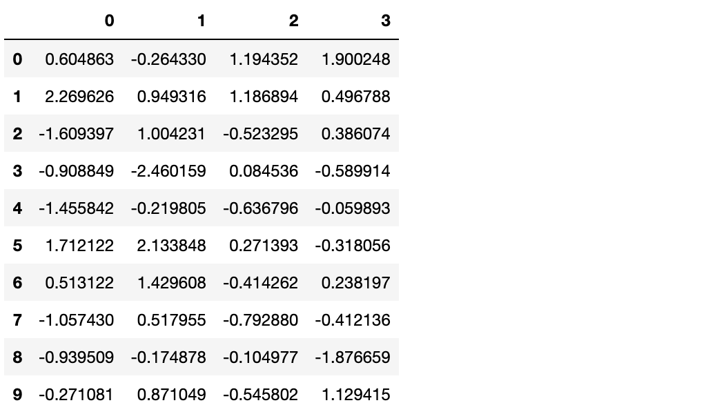
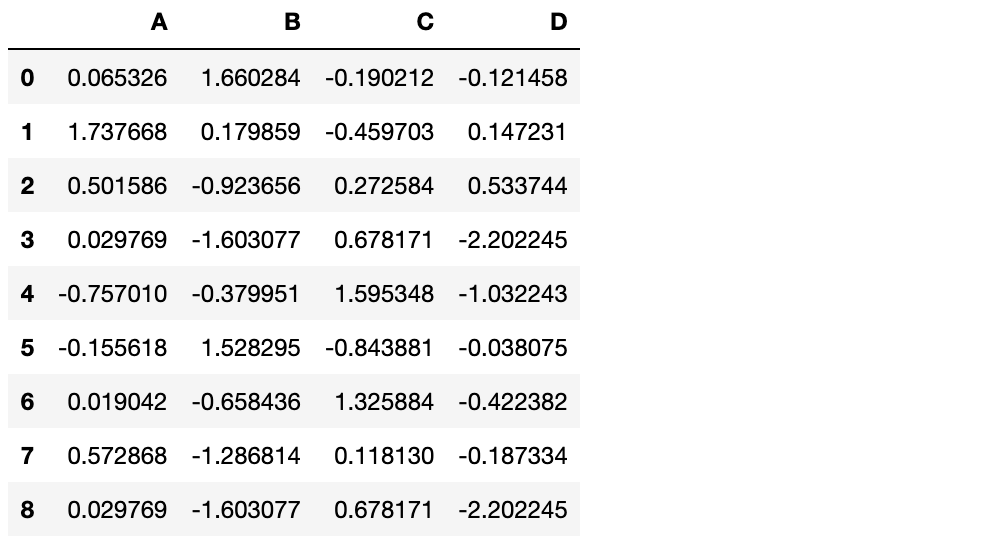
df = pd.DataFrame(np.random.randn(10,4))
df
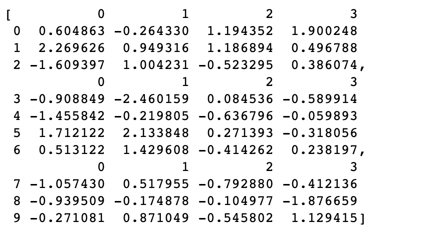
#break it into pieces
pieces = [df[:3], df[3:7], df[7:]]
pieces
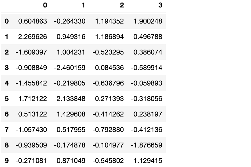
pd.concat(pieces)
Join 合并
类似于SQL中的合并(merge)
left = pd.DataFrame({'key':['foo', 'foo'], 'lval':[1,2]})
left
| key | lval | |
|---|---|---|
| 0 | foo | 1 |
| 1 | foo | 2 |
right = pd.DataFrame({'key':['foo', 'foo'], 'lval':[4,5]})
right
| key | lval | |
|---|---|---|
| 0 | foo | 4 |
| 1 | foo | 5 |
pd.merge(left, right, on='key')
| key | lval_x | lval_y | |
|---|---|---|---|
| 0 | foo | 1 | 4 |
| 1 | foo | 1 | 5 |
| 2 | foo | 2 | 4 |
| 3 | foo | 2 | 5 |
Append 添加
将若干行添加到dataFrame后面
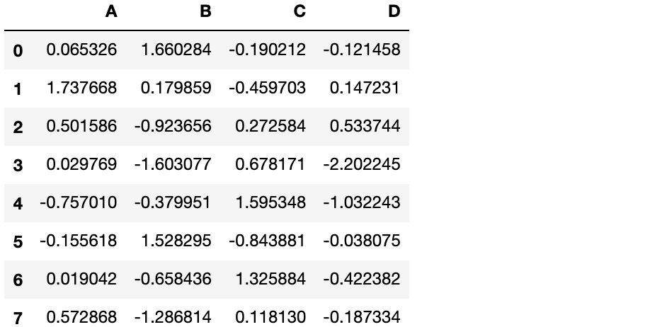
df = pd.DataFrame(np.random.randn(8, 4), columns=['A', 'B', 'C', 'D'])
df
s = df.iloc[3]
s
A    0.163904
B    1.324567
C   -0.768324
D   -0.205520
Name: 3, dtype: float64
df.append(s, ignore_index=True)
分组
对于“group by”操作,我们通常是指以下一个或几个步骤:
划分 按照某些标准将数据分为不同的组 应用 对每组数据分别执行一个函数 组合 将结果组合到一个数据结构
df = pd.DataFrame({'A' : ['foo', 'bar', 'foo', 'bar',
'foo', 'bar', 'foo', 'bar'],
'B' : ['one', 'one', 'two', 'three',
'two', 'two', 'one', 'three'],
'C' : np.random.randn(8),
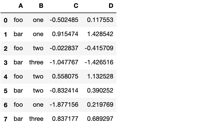
'D' : np.random.randn(8)})
df
分组并对每个分组应用sum函数
df.groupby('A').sum()
| C | D | |
|---|---|---|
| A | ||
| bar | -0.565344 | 1.886637 |
| foo | 2.226542 | 2.122855 |
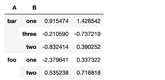
按多个列分组形成层级索引,然后应用函数
df.groupby(['A','B']).sum()
变形
堆叠
tuples = list(zip(*[['bar', 'bar', 'baz', 'baz',
                     'foo', 'foo', 'qux', 'qux'],
                    ['one', 'two', 'one', 'two',
                     'one', 'two', 'one', 'two']]))
index = pd.MultiIndex.from_tuples(tuples, names=['first', 'second'])
df = pd.DataFrame(np.random.randn(8, 2), index=index, columns=['A', 'B'])
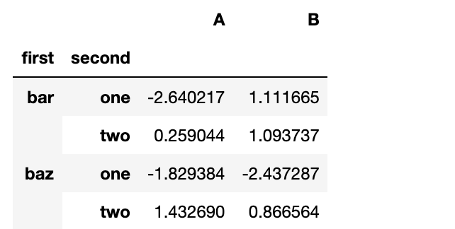
df2 = df[:4]
df2
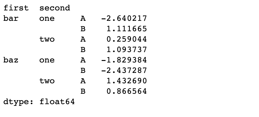
**stack()**方法对DataFrame的列“压缩”一个层级
stacked = df2.stack()
stacked
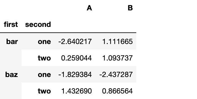
对于一个“堆叠过的”DataFrame或者Series(拥有MultiIndex作为索引),stack()的逆操作是unstack(),默认反堆叠到上一个层级
stacked.unstack()
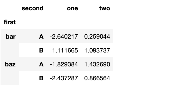
stacked.unstack(1)
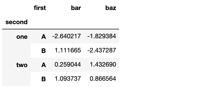
stacked.unstack(0)
数据透视表
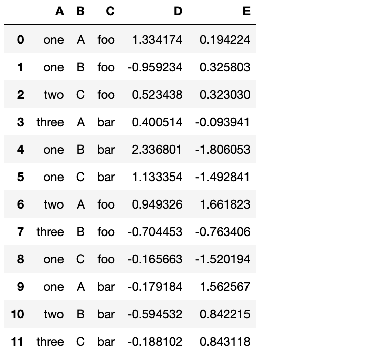
df = pd.DataFrame({'A' : ['one', 'one', 'two', 'three'] * 3,
                   'B' : ['A', 'B', 'C'] * 4,
                   'C' : ['foo', 'foo', 'foo', 'bar', 'bar', 'bar'] * 2,
                   'D' : np.random.randn(12),
                   'E' : np.random.randn(12)})
df
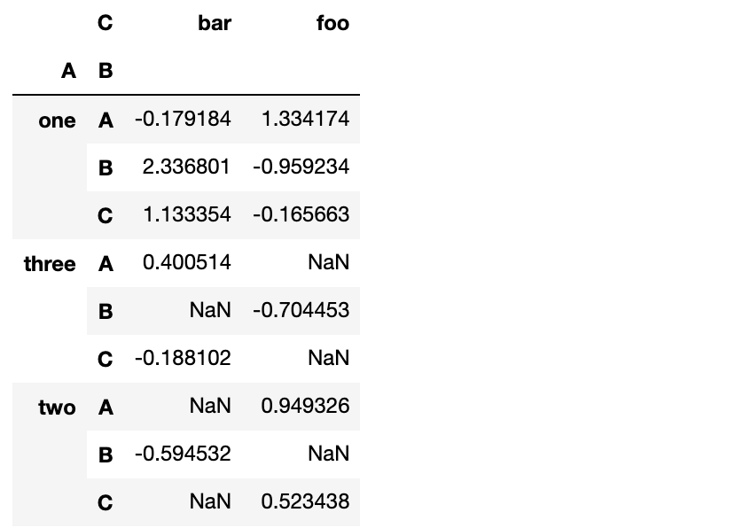
我们可以轻松地从这个数据得到透视表
pd.pivot_table(df, values='D', index=['A', 'B'], columns=['C'])
时间序列
pandas在对频率转换进行重新采样时拥有着简单,强大而且高效的功能(例如把按秒采样的数据转换为按5分钟采样的数据)。这在金融领域很常见,但又不限于此。
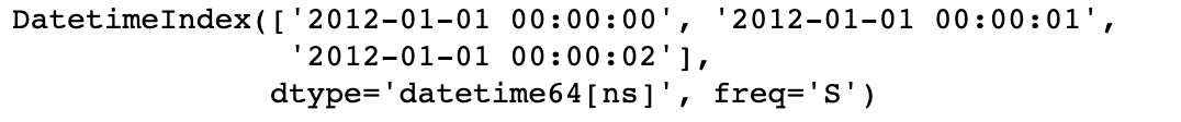
rng = pd.date_range('1/1/2012', periods=100, freq='S')
# 看下前三条DatetimeIndex
rng[0:3]
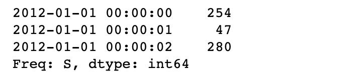
ts = pd.Series(np.random.randint(0,500,len(rng)), index=rng)
# 看下前三条Series数据
ts[0:3]
ts.resample('5Min').sum()
2012-01-01    26203
Freq: 5T, dtype: int32
时区表示
rng = pd.date_range('3/6/2012', periods=5, freq='D')
rng
DatetimeIndex(['2012-03-06', '2012-03-07', '2012-03-08', '2012-03-09',
               '2012-03-10'],
              dtype='datetime64[ns]', freq='D')
ts = pd.Series(np.random.randn(len(rng)), index=rng)
ts
2012-03-06    0.523781
2012-03-07   -0.670822
2012-03-08    0.934826
2012-03-09    0.002239
2012-03-10   -0.091952
Freq: D, dtype: float64
ts_utc = ts.tz_localize('UTC')
ts_utc
2012-03-06 00:00:00+00:00    0.523781
2012-03-07 00:00:00+00:00   -0.670822
2012-03-08 00:00:00+00:00    0.934826
2012-03-09 00:00:00+00:00    0.002239
2012-03-10 00:00:00+00:00   -0.091952
Freq: D, dtype: float64
时区转换
ts_utc.tz_convert('US/Eastern')
2012-03-05 19:00:00-05:00    0.523781
2012-03-06 19:00:00-05:00   -0.670822
2012-03-07 19:00:00-05:00    0.934826
2012-03-08 19:00:00-05:00    0.002239
2012-03-09 19:00:00-05:00   -0.091952
Freq: D, dtype: float64
时间跨度转换
rng = pd.date_range('1/1/2012', periods=5, freq='M')
rng
DatetimeIndex(['2012-01-31', '2012-02-29', '2012-03-31', '2012-04-30',
               '2012-05-31'],
              dtype='datetime64[ns]', freq='M')
ts = pd.Series(np.random.randn(len(rng)), index=rng)
ts
2012-01-31    1.296132
2012-02-29    1.023936
2012-03-31   -0.249774
2012-04-30    1.007810
2012-05-31   -0.051413
Freq: M, dtype: float64
ps = ts.to_period()
ps
2012-01    1.296132
2012-02    1.023936
2012-03   -0.249774
2012-04    1.007810
2012-05   -0.051413
Freq: M, dtype: float64
ps.to_timestamp()
2012-01-01    1.296132
2012-02-01    1.023936
2012-03-01   -0.249774
2012-04-01    1.007810
2012-05-01   -0.051413
Freq: MS, dtype: float64
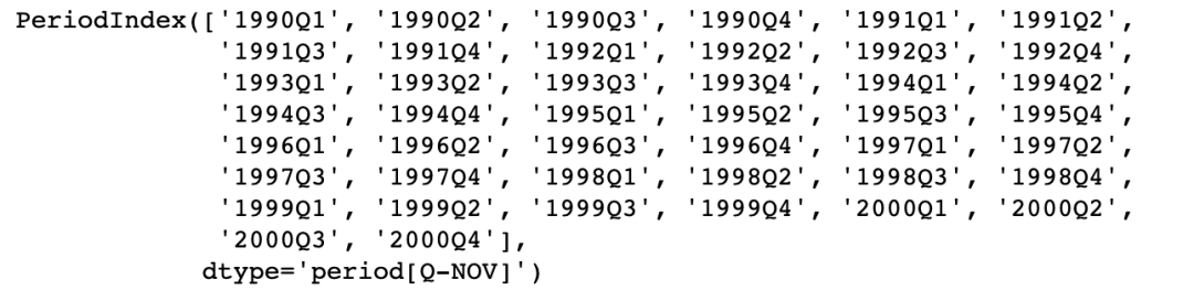
日期与时间戳之间的转换使得可以使用一些方便的算术函数。例如,我们把以11月为年底的季度数据转换为当前季度末月底为始的数据
prng = pd.period_range('1990Q1', '2000Q4', freq='Q-NOV')
prng
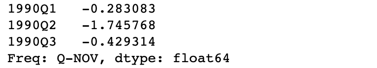
ts = pd.Series(np.random.randn(len(prng)), index = prng)
# 看下数据前三条
ts[0:3]
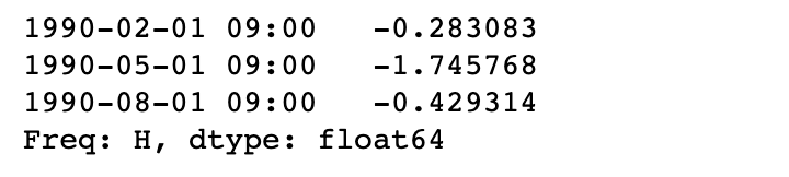
ts.index = (prng.asfreq('M', 'end') ) .asfreq('H', 'start') +9
# 看下数据前三条
ts[0:3]
分类
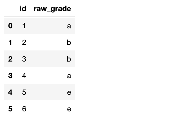
从版本0.15开始,pandas在DataFrame中开始包括分类数据。
df = pd.DataFrame({"id":[1,2,3,4,5,6], "raw_grade":['a', 'b', 'b', 'a', 'e', 'e']})
df
把raw_grade转换为分类类型
df["grade"] = df["raw_grade"].astype("category")
df["grade"]
0    a
1    b
2    b
3    a
4    e
5    e
Name: grade, dtype: category
Categories (3, object): [a, b, e]
重命名类别名为更有意义的名称
df["grade"].cat.categories = ["very good", "good", "very bad"]
对分类重新排序,并添加缺失的分类
df["grade"] = df["grade"].cat.set_categories(["very bad", "bad", "medium", "good", "very good"])
df["grade"]
0    very good
1         good
2         good
3    very good
4     very bad
5     very bad
Name: grade, dtype: category
Categories (5, object): [very bad, bad, medium, good, very good]
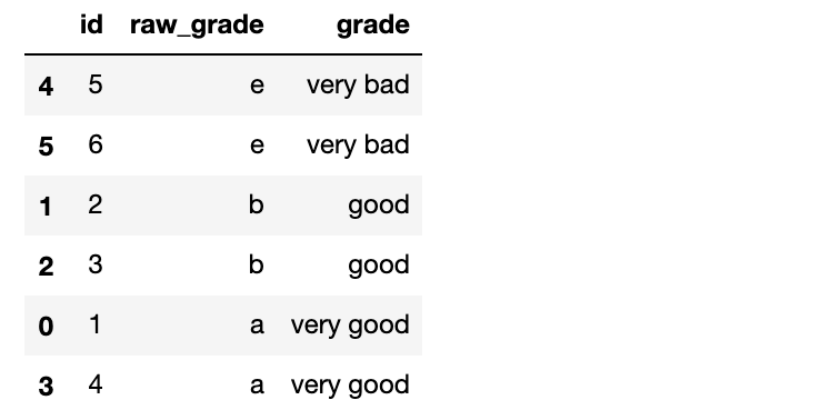
排序是按照分类的顺序进行的,而不是字典序
df.sort_values(by="grade")
按分类分组时,也会显示空的分类
df.groupby("grade").size()
grade
very bad     2
bad          0
medium       0
good         2
very good    2
dtype: int64
绘图
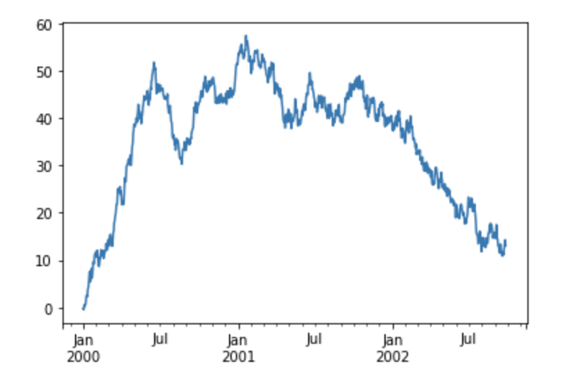
ts = pd.Series(np.random.randn(1000), index=pd.date_range('1/1/2000', periods=1000))
ts = ts.cumsum()
ts.plot()
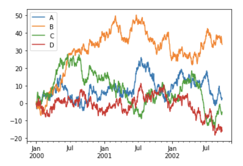
对于DataFrame类型,**plot()**能很方便地画出所有列及其标签
df = pd.DataFrame(np.random.randn(1000, 4), index=ts.index, columns=['A', 'B', 'C', 'D'])
df = df.cumsum()
plt.figure(); df.plot(); plt.legend(loc='best')
获取数据的I/O
CSV
写入一个csv文件
df.to_csv('data/foo.csv')
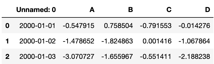
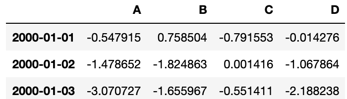
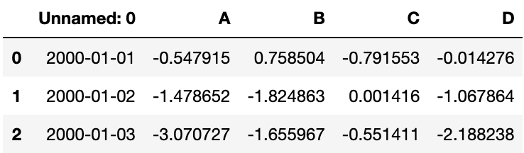
从一个csv文件读入
df1 = pd.read_csv('data/foo.csv')
# 查看前三行数据
df1.head(3)
HDF5
HDFStores的读写
写入一个HDF5 Store
df.to_hdf('data/foo.h5', 'df')
从一个HDF5 Store读入
df1 = pd.read_hdf('data/foo.h5', 'df')
# 查看前三行数据
df1.head(3)
Excel
MS Excel的读写
写入一个Excel文件
df.to_excel('data/foo.xlsx', sheet_name='Sheet1')
从一个excel文件读入
df1 = pd.read_excel('data/foo.xlsx', 'Sheet1', index_col=None, na_values=['NA'])
# 查看前三行数据
df1.head(3)
下期见!
需要本文所有代码和数据的,可以扫下方二维码加我微信后,回复:10pandas 获取。
干货文章,求点赞转发支持。
--END--
扫码即可加我微信
老表朋友圈经常有赠书/红包福利活
如何找到我:
近期优质文章:
学习更多: 整理了我开始分享学习笔记到现在超过250篇优质文章,涵盖数据分析、爬虫、机器学习等方面,别再说不知道该从哪开始,实战哪里找了 “点赞”就是对博主最大的支持